- 1. Planner introduction
- 2. Use cases and examples
- 2.1. Introduction
- 2.2. N queens example
- 2.3. Cloud balancing example
- 2.4. Machine reassignment example (ROADEF 2012)
- 2.5. Manners 2009 example
- 2.6. Traveling Salesman Problem example (TSP)
- 2.7. Traveling Tournament Problem example (TTP)
- 2.8. Curriculum course scheduling example (ITC 2007 track 3)
- 2.9. Examination timetabling example (ITC 2007 track 1)
- 2.10. Patient admission scheduling (hospital bed planning) example (PAS)
- 2.11. Nurse rostering example (INRC 2010)
- 3. Planner configuration
- 4. Score calculation with a rule engine
- 5. Optimization algorithms
- 6. Exact methods
- 7. Construction heuristics
- 8. Local search solver
- 9. Evolutionary algorithms
- 10. Benchmarking and tweaking
- 11. Repeated planning
- Index

Drools Planner optimizes planning problems. It solves use cases, such as:
Employee shift rostering: timetabling nurses, repairmen, ...
Agenda scheduling: scheduling meetings, appointments, maintenance jobs, advertisements, ...
Educational timetabling: scheduling lessons, courses, exams, conference presentations, ...
Vehicle routing: planning vehicles (trucks, trains, boats, airplanes, ...) with freight and/or people
Bin packing: filling containers, trucks, ships and storage warehouses, but also cloud computers nodes, ...
Job shop scheduling: planning car assembly lines, machine queue planning, workforce task planning, ...
Cutting stock: minimizing waste while cutting paper, steel, carpet, ...
Sport scheduling: planning football leagues, baseball leagues, ...
Financial optimization: investment portfolio optimization, risk spreading, ...
Every organization faces planning problems: provide products and services with a limited set of constrained resources (employees, assets, time and money).
Drools Planner enables normal JavaTM programmers to solve planning problems efficiently. Under the hood, it combines optimization algorithms (including Metaheuristics such as Tabu Search and Simulated Annealing) with the power of score calculation by a rule engine.
Drools Planner, like the rest of Drools, is business-friendly open source software under the Apache Software License 2.0 (layman's explanation).
All the use cases above are probably NP-complete. In layman's terms, this means:
It's easy to verify a given solution to a problem in reasonable time.
There is no silver bullet to find the optimal solution of a problem in reasonable time (*).
Note
(*) At least, none of the smartest computer scientists in the world have found such a silver bullet yet. But if they find one for 1 NP-complete problem, it will work for every NP-complete problem.
In fact, there's a $ 1,000,000 reward for anyone that proves if such a silver bullet actually exists or not.
The implication of this is pretty dire: solving your problem is probably harder than you anticipated, because the 2 common techniques won't suffice:
A brute force algorithm (even a smarter variant) will take too long.
A quick algorithm, for example in bin packing, putting in the largest items first, will return a solution that is usually far from optimal.
Drools Planner does find a good solution in reasonable time for such planning problems.
Usually, a planning problem has at least 2 levels of constraints:
A (negative) hard constraint must not be broken. For example: 1 teacher can not teach 2 different lessons at the same time.
A (negative) soft constraint should not be broken if it can be avoided. For example: Teacher A does not like to teach on Friday afternoon.
Some problems have positive constraints too:
A positive soft constraint (or reward) should be fulfilled if possible. For example: Teacher B likes to teach on Monday morning.
In practice, these are just like negative soft constraints, but with a positive weight.
Some toy problems (such as N Queens) only have hard constraints. Some problems have 3 or more levels of constraints, for example hard, medium and soft constraints.
These constraints define the score function (AKA fitness function) of a planning problem. Each solution of a planning problem can be graded with a score. Because we 'll define these constraints as rules in the Drools Expert rule engine, adding constraints in Drools Planner is easy and scalable.
A planning problem has a number of solutions. There are several categories of solutions:
A possible solution is a solution that does or does not break any number of constraints. Planning problems tend to have a incredibly large number of possible solutions. Most of those solutions are worthless.
A feasible solution is a solution that does not break any (negative) hard constraints. The number of feasible solutions tends to be relative to the number of possible solutions. Sometimes there are no feasible solutions. Every feasible solution is a possible solution.
An optimal solution is a solution with the highest score. Planning problems tend to have 1 or a few optimal solutions. There is always at least 1 optimal solution, even in the case that there are no feasible solutions and the optimal solution isn't feasible.
The best solution found is the solution with the highest score found by an implementation in a given amount of time. The best solution found is likely to be feasible.
Counterintuitively, the number of possible solutions is huge (if calculated correctly), even with a small dataset. As you'll see in the examples, most instances have a lot more possible solutions than the minimal number of atoms in the known universe (10^80). Because there is no silver bullet to find the optimal solution, any implementation is forced to evaluate at least a subset of all those possible solutions.
Drools Planner supports several optimization algorithms to efficiently wade through that incredibly large number of possible solutions. Depending on the use case, some optimization algorithms perform better than others. In Drools Planner it is easy to switch the optimization algorithm, by changing the solver configuration in a few XML lines or by API.
Drools Planner is production ready. The API is almost stable but backward incompatible changes can occur. With
the recipe called UpgradeFromPreviousVersionRecipe.txt
you can easily upgrade and deal with any backwards incompatible changes between versions. That recipe file is
included in every release.
You can download a release zip of Drools Planner from the Drools download site. Unzip it. To run an
example, just open the directory examples and run the script
(runExamples.sh on Linux and Mac or runExamples.bat on Windows) and pick
an example in the GUI:
$ cd examples
$ ./runExamples.sh
$ cd examples
$ runExamples.bat
To run the examples in your favorite IDE, first configure your IDE:
In IntelliJ and NetBeans, just open the file
examples/sources/pom.xmlas a new project, the maven integration will take care of the rest.In Eclipse, open a new project for the directory
examples/sources.Add all the jars to the classpath from the directory
binariesand the directoryexamples/binaries, except for the fileexamples/binaries/drools-planner-examples-*.jar.Add the java source directory
src/main/javaand the java resources directorysrc/main/resources.
Next, create a run configuration:
Main class:
org.drools.planner.examples.app.DroolsPlannerExamplesAppVM parameters (optional):
-Xmx512M -serverWorking directory:
examples(this is the directory that contains the directorydata)
The Drools Planner jars are available on the central maven repository (and the JBoss maven repository).
If you use maven, just add a dependency to drools-planner-core in your project's
pom.xml:
    <dependency>

        <groupId>org.drools.planner</groupId>

        <artifactId>drools-planner-core</artifactId>

        <version>5.x</version>

    </dependency>
This is similar for gradle, ivy and buildr.
If you're still using ant (without ivy), copy all the jars from the download zip's
binaries directory and manually verify that your classpath doesn't contain duplicate
jars.
You can also easily build it from source yourself.
Set up Git and clone
drools-planner from GitHub (or alternatively, download the zipball):
$ git clone git@github.com:droolsjbpm/drools-planner.git drools-planner
...
Then do a Maven 3 build:
$ cd drools-planner
$ mvn -DskipTests clean install
...
After that, you can run any example directly from the command line, just run this command and pick an example:
$ cd drools-planner-examples
$ mvn exec:exec
...
Your questions and comments are welcome on the user
mailing list. Start the subject of your mail with [planner]. You can read/write to the
user mailing list without littering your mailbox through this web forum or this newsgroup.
Feel free to report an issue (such as a bug, improvement or a new feature request) for the Drools Planner code
or for this manual to the drools issue tracker.
Select the component drools-planner.
Pull requests (and patches) are very welcome and get priority treatment! Include the pull request link to a JIRA issue and optionally send a mail to the dev mailing list to get the issue fixed fast. By open sourcing your improvements, you 'll benefit from our peer review, improvements made upon your improvements and maybe even a thank you on our blog.
Check our blog and twitter (Geoffrey De Smet) for news and articles. If Drools Planner helps you solve your problem, don't forget to blog or tweet about it!
- 2.1. Introduction
- 2.2. N queens example
- 2.3. Cloud balancing example
- 2.4. Machine reassignment example (ROADEF 2012)
- 2.5. Manners 2009 example
- 2.6. Traveling Salesman Problem example (TSP)
- 2.7. Traveling Tournament Problem example (TTP)
- 2.8. Curriculum course scheduling example (ITC 2007 track 3)
- 2.9. Examination timetabling example (ITC 2007 track 1)
- 2.10. Patient admission scheduling (hospital bed planning) example (PAS)
- 2.11. Nurse rostering example (INRC 2010)
Drools Planner has several examples. In this manual we explain Drools Planner mainly using the n queens example. So it's advisable to read at least the section about that example. For advanced users, the following examples are recommended: curriculum course and nurse rostering.
You can find the source code of all these examples in the distribution zip under
examples/sources and also in git under
drools-planner/drools-planner-examples.
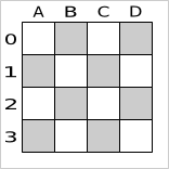
The n queens puzzle is a puzzle with the following constraints:
Use a chessboard of n columns and n rows.
Place n queens on the chessboard.
No 2 queens can attack each other. Note that a queen can attack any other queen on the same horizontal, vertical or diagonal line.
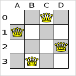
The most common n queens puzzle is the 8 queens puzzle, with n = 8. We 'll explain Drools Planner using the 4 queens puzzle as the primary example.
A proposed solution could be:
The above solution is wrong because queens A1 and B0 can attack each
other (as can queens B0 and D0). Removing queen B0 would
respect the "no 2 queens can attack each other" constraint, but would break the "place n queens"
constraint.
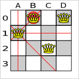
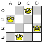
Below is a correct solution:
All the constraints have been met, so the solution is correct. Note that most n queens puzzles have multiple correct solutions. We 'll focus on finding a single correct solution for a given n, not on finding the number of possible correct solutions for a given n.
These numbers might give you some insight on the size of this problem.
Table 2.1. NQueens problem size
| # queens (n) | # possible solutions (each queen its own column) | # feasible solutions (= optimal in this use case) | # optimal solutions | # optimal out of # possible |
|---|---|---|---|---|
| 4 | 256 | 2 | 2 | 1 out of 128 |
| 8 | 16777216 | 64 | 64 | 1 out of 262144 |
| 16 | 18446744073709551616 | 14772512 | 14772512 | 1 out of 1248720872503 |
| 32 | 1.46150163733090291820368483e+48 | ? | ? | ? |
| 64 | 3.94020061963944792122790401e+115 | ? | ? | ? |
| n | n ^ n | ? | # feasible solutions | ? |
The Drools Planner implementation has not been optimized because it functions as a beginner example. Nevertheless, it can easily handle 64 queens.
Use a good domain model: it will be easier to understand and solve your planning problem with Drools Planner. This is the domain model for the n queens example:
public class Column {

    private int index;

    // ... getters and setters
}
public class Row {
private int index;
// ... getters and setters
}public class Queen {
private Column column;
private Row row;
public int getAscendingDiagonalIndex() {...}
public int getDescendingDiagonalIndex() {...}
// ... getters and setters
}public class NQueens implements Solution<SimpleScore> {
private int n;
private List<Column> columnList;
private List<Row> rowList;
private List<Queen> queenList;
private SimpleScore score;
// ... getters and setters
}A Queen instance has a Column (for example: 0 is column A, 1 is column
B, ...) and a Row (its row, for example: 0 is row 0, 1 is row 1, ...). Based on the column and
the row, the ascending diagonal line as well as the descending diagonal line can be calculated. The column and row
indexes start from the upper left corner of the chessboard.
Table 2.2. A solution for the 4 queens puzzle shown in the domain model
| A solution | Queen | columnIndex | rowIndex | ascendingDiagonalIndex (columnIndex + rowIndex) | descendingDiagonalIndex (columnIndex - rowIndex) |
|---|---|---|---|---|---|
 | A1 | 0 | 1 | 1 (**) | -1 |
| B0 | 1 | 0 (*) | 1 (**) | 1 | |
| C2 | 2 | 2 | 4 | 0 | |
| D0 | 3 | 0 (*) | 3 | 3 |
When 2 queens share the same column, row or diagonal line, such as (*) and (**), they can attack each other.
A single NQueens instance contains a list of all Queen instances. It
is the Solution implementation which will be supplied to, solved by and retrieved from the
Solver. Notice that in the 4 queens example, NQueens's getN() method will always return
4.
Assign each process to a server.
Hard constraints:
Every server should be able to handle the sum of each of the minimal hardware requirements (CPR, RAM, network bandwidth) of all its processes.
Soft constraints:
Each server that has one or more processes assigned, has a fixed maintenance cost. Minimize the total cost.
This is a form of bin packing.


Assign each process to a machine. All processes already have an original (unoptimized) assignment. Each process requires an amount of each resource (such as CPU, RAM, ...). This is more complex version of the Cloud balancing example.
The problem is defined by the Google ROADEF/EURO Challenge 2012.
Hard constraints:
Maximum capacity: The maximum capacity for each resource for each machine must not be exceeded.
Conflict: Processes of the same service must run on distinct machines.
Spread: Processes of the same service must be spread across locations.
Dependency: The processes of a service depending on another service must run in the neighborhood of a process of the other service.
Transient usage: Some resources are transient and count towards the maximum capacity of both the original machine as the newly assigned machine.
Soft constraints:
Load: The safety capacity for each resource for each machine should not be exceeded.
Balance: Leave room for future assignments by balancing the available resources on each machine.
Process move cost: A process has a move cost.
Service move cost: A service has a move cost.
Machine move cost: Moving a process from machine A to machine B has another A-B specific move cost.
model_a1_1: 2 resources, 1 neighborhoods, 4 locations, 4 machines, 79 services, 100 processes and 1 balancePenalties with flooredPossibleSolutionSize (10^60).
model_a1_2: 4 resources, 2 neighborhoods, 4 locations, 100 machines, 980 services, 1000 processes and 0 balancePenalties with flooredPossibleSolutionSize (10^2000).
model_a1_3: 3 resources, 5 neighborhoods, 25 locations, 100 machines, 216 services, 1000 processes and 0 balancePenalties with flooredPossibleSolutionSize (10^2000).
model_a1_4: 3 resources, 50 neighborhoods, 50 locations, 50 machines, 142 services, 1000 processes and 1 balancePenalties with flooredPossibleSolutionSize (10^1698).
model_a1_5: 4 resources, 2 neighborhoods, 4 locations, 12 machines, 981 services, 1000 processes and 1 balancePenalties with flooredPossibleSolutionSize (10^1079).
model_a2_1: 3 resources, 1 neighborhoods, 1 locations, 100 machines, 1000 services, 1000 processes and 0 balancePenalties with flooredPossibleSolutionSize (10^2000).
model_a2_2: 12 resources, 5 neighborhoods, 25 locations, 100 machines, 170 services, 1000 processes and 0 balancePenalties with flooredPossibleSolutionSize (10^2000).
model_a2_3: 12 resources, 5 neighborhoods, 25 locations, 100 machines, 129 services, 1000 processes and 0 balancePenalties with flooredPossibleSolutionSize (10^2000).
model_a2_4: 12 resources, 5 neighborhoods, 25 locations, 50 machines, 180 services, 1000 processes and 1 balancePenalties with flooredPossibleSolutionSize (10^1698).
model_a2_5: 12 resources, 5 neighborhoods, 25 locations, 50 machines, 153 services, 1000 processes and 0 balancePenalties with flooredPossibleSolutionSize (10^1698).
In Manners 2009, miss Manners is throwing a party again.
This time she invited 144 guests and prepared 12 round tables with 12 seats each.
Every guest should sit next to someone (left and right) of the opposite gender.
And that neighbour should have at least one hobby in common with the guest.
Also, this time there should be 2 politicians, 2 doctors, 2 socialites, 2 sports stars, 2 teachers and 2 programmers at each table.
And the 2 politicians, 2 doctors, 2 sports stars and 2 programmers shouldn't be the same kind.
Drools Expert also has the normal miss Manners examples (which is much smaller) and employs a brute force heuristic to solve it. Drools Planner's implementation employs far more scalable heuristics while still using Drools Expert to calculate the score..
Given a list of cities, find the shortest tour for a salesman that visits each city exactly once. See the wikipedia definition of the traveling Salesman Problem.
It is one of the most intensively studied problems in computational mathematics. Yet, in the real world, it's often only part of a planning problem, along with other constraints, such as employee shift time constraints.
Schedule matches between n teams with the following hard constraints:
Each team plays twice against every other team: once home and once away.
Each team has exactly 1 match on each timeslot.
No team must have more than 3 consecutive home or 3 consecutive away matches.
No repeaters: no 2 consecutive matches of the same 2 opposing teams.
and the following soft constraint:
Minimize the total distance traveled by all teams.
The problem is defined on Michael Trick's website (which contains several world records too).

There are 2 implementations (simple and smart) to demonstrate the importance of some performance tips. The
DroolsPlannerExamplesApp always runs the smart implementation, but with these commands you can
compare the 2 implementations yourself:
$ mvn exec:exec -Dexec.mainClass="org.drools.planner.examples.travelingtournament.app.simple.SimpleTravelingTournamentApp"
...
$ mvn exec:exec -Dexec.mainClass="org.drools.planner.examples.travelingtournament.app.smart.SmartTravelingTournamentApp"
...
The smart implementation performs and scales exponentially better than the simple implementation.
These numbers might give you some insight on the size of this problem.
Table 2.3. Traveling tournament problem size
| # teams | # days | # matches | # possible solutions (simple) | # possible solutions (smart) | # feasible solutions | # optimal solutions |
|---|---|---|---|---|---|---|
| 4 | 6 | 12 | 2176782336 | <= 518400 | ? | 1? |
| 6 | 10 | 30 | 1000000000000000000000000000000 | <= 47784725839872000000 | ? | 1? |
| 8 | 14 | 56 | 1.52464943788290465606136043e+64 | <= 5.77608277425558771434498864e+43 | ? | 1? |
| 10 | 18 | 90 | 9.43029892325559280477052413e+112 | <= 1.07573451027871200629339068e+79 | ? | 1? |
| 12 | 22 | 132 | 1.58414112478195320415135060e+177 | <= 2.01650616733413376416949843e+126 | ? | 1? |
| 14 | 26 | 182 | 3.35080635695103223315189511e+257 | <= 1.73513467024013808570420241e+186 | ? | 1? |
| 16 | 30 | 240 | 3.22924601799855400751522483e+354 | <= 2.45064610271441678267620602e+259 | ? | 1? |
| n | 2 * (n - 1) | n * (n - 1) | (2 * (n - 1)) ^ (n * (n - 1)) | <= (((2 * (n - 1))!) ^ (n / 2)) | ? | 1? |
Schedule each lecture into a timeslot and into a room.
The problem is defined by the International Timetabling Competition 2007 track 3.
Schedule each exam into a period and into a room. Multiple exams can share the same room during the same period.
There are a number of hard constraints that cannot be broken:
Exam conflict: 2 exams that share students should not occur in the same period.
Room capacity: A room's seating capacity should suffice at all times.
Period duration: A period's duration should suffice for all of its exams.
Period related hard constraints should be fulfilled:
Coincidence: 2 exams should use the same period (but possibly another room).
Exclusion: 2 exams should not use the same period.
After: 1 exam should occur in a period after another exam's period.
Room related hard constraints should be fulfilled:
Exclusive: 1 exam should not have to share its room with any other exam.
There are also a number of soft constraints that should be minimized (each of which has parameterized penalty's):
2 exams in a row.
2 exams in a day.
Period spread: 2 exams that share students should be a number of periods apart.
Mixed durations: 2 exams that share a room should not have different durations.
Front load: Large exams should be scheduled earlier in the schedule.
Period penalty: Some periods have a penalty when used.
Room penalty: Some rooms have a penalty when used.
It uses large test data sets of real-life universities.
The problem is defined by the International Timetabling Competition 2007 track 1.

These numbers might give you some insight on the size of this problem.
Table 2.4. Examination problem size
| Set | # students | # exams/topics | # periods | # rooms | # possible solutions | # feasible solutions | # optimal solutions |
|---|---|---|---|---|---|---|---|
| exam_comp_set1 | 7883 | 607 | 54 | 7 | 10^1564 | ? | 1? |
| exam_comp_set2 | 12484 | 870 | 40 | 49 | 10^2864 | ? | 1? |
| exam_comp_set3 | 16365 | 934 | 36 | 48 | 10^3023 | ? | 1? |
| exam_comp_set4 | 4421 | 273 | 21 | 1 | 10^360 | ? | 1? |
| exam_comp_set5 | 8719 | 1018 | 42 | 3 | 10^2138 | ? | 1? |
| exam_comp_set6 | 7909 | 242 | 16 | 8 | 10^509 | ? | 1? |
| exam_comp_set7 | 13795 | 1096 | 80 | 28 | 10^3671 | ? | 1? |
| exam_comp_set8 | 7718 | 598 | 80 | 8 | 10^1678 | ? | 1? |
| ? | s | t | p | r | (p * r) ^ e | ? | 1? |
Geoffrey De Smet (the Drools Planner lead) finished 4th in the International Timetabling Competition 2007's examination track with a very early version of Drools Planner. Many improvements have been made since then.
Below you can see the main examination domain classes:
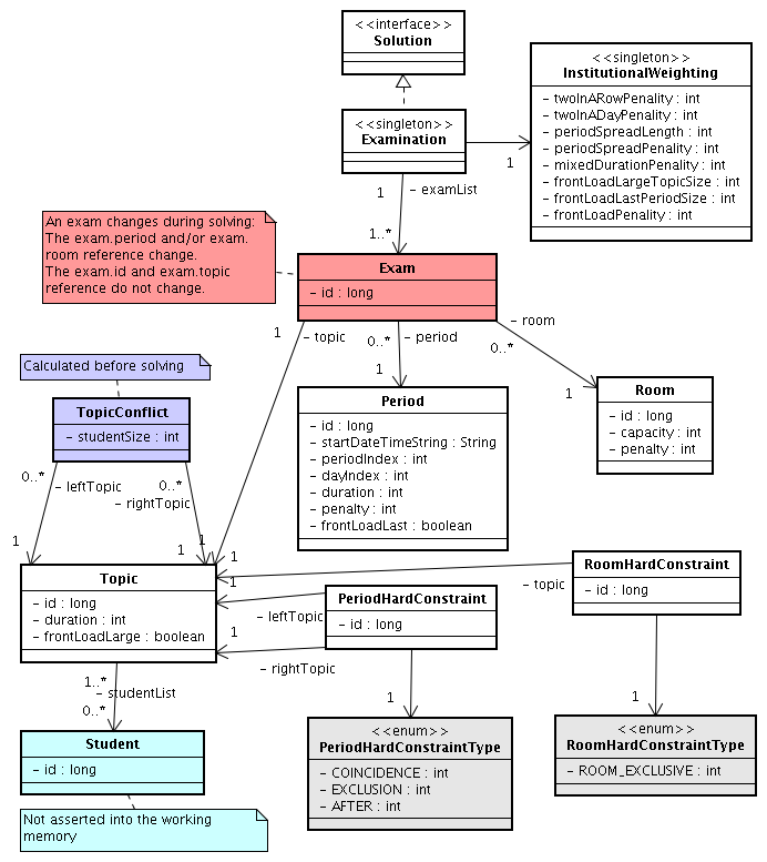
Notice that we've split up the exam concept into an Exam class and a
Topic class. The Exam instances change during solving (this is the planning
entity class), when they get another period or room property. The Topic,
Period and Room instances never change during solving (these are problem
facts, just like some other classes).
Assign each patient (that will come to the hospital) into a bed for each night that the patient will stay in the hospital. Each bed belongs to a room and each room belongs to a department. The arrival and departure dates of the patients is fixed: only a bed needs to be assigned for each night.
There are a couple of hard constraints:
2 patients shouldn't be assigned to the same bed in the same night.
A room can have a gender limitation: only females, only males, the same gender in the same night or no gender limitation at all.
A department can have a minimum or maximum age.
A patient can require a room with specific equipment(s).
And of course, there are also some soft constraints:
A patient can prefer a maximum room size, for example if he/she want a single room.
A patient is best assigned to a department that specializes in his/her problem.
A patient is best assigned to a room that specializes in his/her problem.
A patient can prefer a room with specific equipment(s).
The problem is defined on this webpage and the test data comes from real world hospitals.

For each shift, assign a nurse to work that shift.
The problem is defined by the International Nurse Rostering Competition 2010.


Solving a planning problem with Drools Planner consists out of 5 steps:
Model your planning problem as a class that implements the interface
Solution, for example the classNQueens.Configure a
Solver, for example a first fit and tabu search solver for anyNQueensinstance.Load a problem data set from your data layer, for example a 4 Queens instance. Set it as the planning problem on the
SolverwithSolver.setPlanningProblem(...).Solve it with
Solver.solve().Get the best solution found by the
SolverwithSolver.getBestSolution().
You can build a Solver instance with the XmlSolverConfigurer.
Configure it with a solver configuration XML file:
        XmlSolverConfigurer configurer = new XmlSolverConfigurer();

        configurer.configure("/org/drools/planner/examples/nqueens/solver/nqueensSolverConfig.xml");

        Solver solver = configurer.buildSolver();
A solver configuration file looks something like this:
<?xml version="1.0" encoding="UTF-8"?>

<solver>

  <!-- Define the model -->

  <solutionClass>org.drools.planner.examples.nqueens.domain.NQueens</solutionClass>

  <planningEntityClass>org.drools.planner.examples.nqueens.domain.Queen</planningEntityClass>


  <!-- Define the score function -->

  <scoreDrl>/org/drools/planner/examples/nqueens/solver/nQueensScoreRules.drl</scoreDrl>

  <scoreDefinition>

    <scoreDefinitionType>SIMPLE</scoreDefinitionType>

  </scoreDefinition>


  <!-- Configure the optimization algorithm(s) -->

  <termination>

    ...

  </termination>

  <constructionHeuristic>

    ...

  </constructionHeuristic>

  <localSearch>

    ...

  </localSearch>

</solver>
Notice the 3 parts in it:
Define the model
Define the score function
Configure the optimization algorithm(s)
We 'll explain these various parts of a configuration later in this manual.
Drools Planner makes it relatively easy to switch optimization algorithm(s) just by
changing the configuration. There's even a Benchmark utility which allows you to
play out different configurations against each other and report the most appropriate configuration for your
problem. You could for example play out tabu search versus simulated annealing, on 4 queens and 64 queens.
As an alternative to the XML file, a solver configuration can also be configured with the
SolverConfig API:
        SolverConfig solverConfig = new SolverConfig();

        solverConfig.setSolutionClass(NQueens.class);
        Set<Class<?>> planningEntityClassSet = new HashSet<Class<?>>();
        planningEntityClassSet.add(Queen.class);
        solverConfig.setPlanningEntityClassSet(planningEntityClassSet);

        solverConfig.setScoreDrlList(
                Arrays.asList("/org/drools/planner/examples/nqueens/solver/nQueensScoreRules.drl"));
        ScoreDefinitionConfig scoreDefinitionConfig = solverConfig.getScoreDefinitionConfig();
        scoreDefinitionConfig.setScoreDefinitionType(
                ScoreDefinitionConfig.ScoreDefinitionType.SIMPLE);

        TerminationConfig terminationConfig = solverConfig.getTerminationConfig();
        // ...
        List<SolverPhaseConfig> solverPhaseConfigList = new ArrayList<SolverPhaseConfig>();
        ConstructionHeuristicSolverPhaseConfig constructionHeuristicSolverPhaseConfig
                = new ConstructionHeuristicSolverPhaseConfig();
        // ...
        solverPhaseConfigList.add(constructionHeuristicSolverPhaseConfig);
        LocalSearchSolverPhaseConfig localSearchSolverPhaseConfig = new LocalSearchSolverPhaseConfig();
        // ...
        solverPhaseConfigList.add(localSearchSolverPhaseConfig);
        solverConfig.setSolverPhaseConfigList(solverPhaseConfigList);
        Solver solver = solverConfig.buildSolver();
It is highly recommended to configure by XML file instead of this API. To
dynamically configure a value at runtime, use the XML file as a template and extract the
SolverConfig class with getSolverConfig() to configure the dynamic value at
runtime:
        XmlSolverConfigurer configurer = new XmlSolverConfigurer();
        configurer.configure("/org/drools/planner/examples/nqueens/solver/nqueensSolverConfig.xml");

        SolverConfig solverConfig = configurer.getSolverConfig();
        solverConfig.getTerminationConfig().setMaximumMinutesSpend(userInput);
Solver solver = solverConfig.buildSolver();Look at a dataset of your planning problem. You 'll recognize domain classes in there, each of which is one of these:
A unrelated class: not used by any of the score constraints. From a planning standpoint, this data is obsolete.
A problem fact class: used by the score constraints, but does NOT change during planning (as long as the problem stays the same). For example:
Bed,Room,Shift,Employee,Topic,Period, ...A planning entity class: used by the score constraints and changes during planning. For example:
BedDesignation,ShiftAssignment,Exam, ...
Ask yourself: What class changes during planning? Which class has variables
that I want the Solver to choose for me? That class is a planning entity. Most use
cases have only 1 planning entity class.
Note
In real-time planning, problem facts can change during planning, because the problem itself changes. However, that doesn't make them planning entities.
In Drools Planner all problems facts and planning entities are plain old JavaBeans (POJO's). You can load them from a database (JDBC/JPA/JDO), an XML file, a data repository, a noSQL cloud, ...: Drools Planner doesn't care.
A problem fact is any JavaBean (POJO) with getters that does not change during planning. Implementing the
interface Serializable is recommended (but not required). For example in n queens, the columns
and rows are problem facts:
public class Column implements Serializable {

    private int index;

    // ... getters
}
public class Row implements Serializable {
private int index;
// ... getters
}A problem fact can reference other problem facts of course:
public class Course implements Serializable {

    private String code;

    private Teacher teacher; // Other problem fact
    private int lectureSize;
    private int minWorkingDaySize;

    private List<Curriculum> curriculumList; // Other problem facts
    private int studentSize;

    // ... getters
}
A problem fact class does not require any Planner specific code. For example, you can reuse your domain classes, which might have JPA annotations.
Note
Generally, better designed domain classes lead to simpler and more efficient score constraints. Therefore,
when dealing with a messy legacy system, it can sometimes be worth it to convert the messy domain set into a
planner specific POJO set first. For example: if your domain model has 2 Teacher instances
for the same teacher that teaches at 2 different departments, it's hard to write a correct score constraint that
constrains a teacher's spare time.
Alternatively, you can sometimes also introduce a cached problem fact to enrich the domain model for planning only.
A planning entity is a JavaBean (POJO) that changes during solving, for example a Queen
that changes to another row. A planning problem has multiple planning entities, for example for a single n
queens problem, each Queen is a planning entity. But there's usually only 1 planning entity
class, for example the Queen class.
A planning entity class needs to be annotated with the @PlanningEntity
annotation.
Each planning entity class has 1 or more planning variables. It usually also has 1 or
more defining properties. For example in n queens, a Queen is defined by
it's Column and has a planning variable Row. This means that a Queen's
column never changes during solving, while it's row does change.
@PlanningEntity
public class Queen {

    private Column column;

    // Planning variables: changes during planning, between score calculations.
    private Row row;

    // ... getters and setters
}
A planning entity class can have multiple planning variables. For example, a Lecture is
defined by it's Course and it's index in that course (because 1 course has multiple
lectures). Each Lecture needs to be scheduled into a Period and a
Room so it has 2 planning variables (period and room). For example: the course Mathematics
has 8 lectures per week, of which the first lecture is Monday morning at 08:00 in room 212.
@PlanningEntity
public class Lecture {

    private Course course;
    private int lectureIndexInCourse;

    // Planning variables: changes during planning, between score calculations.
    private Period period;
    private Room room;

    // ...
}
The solver configuration also needs to be made aware of each planning entity class:
<solver>
  ...
  <planningEntityClass>org.drools.planner.examples.nqueens.domain.Queen</planningEntityClass>
  ...
</solver>
Some uses cases have multiple planning entity classes. For example: route freight and trains into railway network arcs, where each freight can use multiple trains over it's journey and each train can carry multiple freights per arc. Having multiple planning entity classes directly raises the implementation complexity of your use case.
Note
Do not create unnecessary planning entity classes. This leads to difficult
Move implementations and slower score calculation.
For example, do not create a planning entity class to hold the total free time of a teacher, which needs
to be kept up to date as the Lecture planning entities change. Instead, calculate the free
time in the score constraints and put the result per teacher into a logically inserted score object.
If historic data needs to be considered too, then create problem fact to hold the historic data up to, but not including, the planning window (so it doesn't change when a planning entity changes) and let the score constraints take it into account.
Some optimization algorithms work more efficiently if they have an estimation of which planning entities are more difficult to plan. For example: in bin packing bigger items are harder to fit, in course scheduling lectures with more students are more difficult to schedule and in n queens the middle queens are more difficult.
Therefore, you can set a difficultyComparatorClass to the
@PlanningEntity annotation:
@PlanningEntity(difficultyComparatorClass = CloudProcessAssignmentDifficultyComparator.class)
public class CloudProcessAssignment {
    // ...
}
public class CloudProcessAssignmentDifficultyComparator implements Comparator<CloudProcessAssignment> {
public int compare(CloudProcessAssignment a, CloudProcessAssignment b) {
return new CompareToBuilder()
.append(a.getCloudProcess().getRequiredMultiplicand(), b.getCloudProcess().getRequiredMultiplicand())
.append(a.getCloudProcess().getId(), b.getCloudProcess().getId())
.toComparison();
}
}Note
If you have multiple planning entity classes, the difficultyComparatorClass needs to
implement a Comparator of a common superclass (for example
Comparator<Object>) and be able to handle comparing instances of those different
classes.
Alternatively, you can also set a difficultyWeightFactoryClass to the
@PlanningEntity annotation, so you have access to the rest of the problem facts from the
solution too:
@PlanningEntity(difficultyWeightFactoryClass = QueenDifficultyWeightFactory.class)
public class Queen {
    // ...
}
public interface PlanningEntityDifficultyWeightFactory {
Comparable createDifficultyWeight(Solution solution, Object planningEntity);
}public class QueenDifficultyWeightFactory implements PlanningEntityDifficultyWeightFactory {
public Comparable createDifficultyWeight(Solution solution, Object planningEntity) {
NQueens nQueens = (NQueens) solution;
Queen queen = (Queen) planningEntity;
int distanceFromMiddle = calculateDistanceFromMiddle(nQueens.getN(), queen.getColumnIndex());
return new QueenDifficultyWeight(queen, distanceFromMiddle);
}
// ...
public static class QueenDifficultyWeight implements Comparable<QueenDifficultyWeight> {
private final Queen queen;
private final int distanceFromMiddle;
public QueenDifficultyWeight(Queen queen, int distanceFromMiddle) {
this.queen = queen;
this.distanceFromMiddle = distanceFromMiddle;
}
public int compareTo(QueenDifficultyWeight other) {
return new CompareToBuilder()
// The more difficult queens have a lower distance to the middle
.append(other.distanceFromMiddle, distanceFromMiddle) // Decreasing
.append(queen.getColumnIndex(), other.queen.getColumnIndex())
.toComparison();
}
}
}None of the current planning variable state may be used to compare planning entities.
They are likely to be null anyway. For example, a Queen's
row variable may not be used.
A planning variable is a property (including getter and setter) on a planning entity. It changes during
planning. For example, a Queen's row property is a planning variable. Note
that even though a Queen's row property changes to another
Row during planning, no Row instance itself is changed. A planning
variable points to a planning value.
A planning variable getter needs to be annotated with the @PlanningVariable annotation.
Furthermore, it needs a @ValueRange* annotation too.
@PlanningEntity
public class Queen {

    private Row row;

    // ...

    @PlanningVariable
    @ValueRangeFromSolutionProperty(propertyName = "rowList")
    public Row getRow() {
        return row;
    }

    public void setRow(Row row) {
        this.row = row;
    }

}A planning value is a possible value for a planning variable. Usually, a planning value is problem fact, but it can also be any object, for example a double. Sometimes it can even be another planning entity.
A planning value range is the set of possible planning values for a planning variable. This set can be a
discrete (for example row 1, 2, 3 or
4) or continuous (for example any double between 0.0
and 1.0). There are several ways to define the value range of a planning variable, each with
it's own @ValueRange* annotation.
If null is a valid planning value, it should be included in the value range and the
default way to detect uninitialized planning variables must be changed.
All instances of the same planning entity class share the same set of possible planning values for that planning variable. This is the most common way to configure a value range.
The Solution implementation has property which returns a
Collection. Any value from that Collection is a possible planning value
for this planning variable.
    @PlanningVariable
    @ValueRangeFromSolutionProperty(propertyName = "rowList")
    public Row getRow() {
        return row;
    }
public class NQueens implements Solution<SimpleScore> {
// ...
public List<Row> getRowList() {
return rowList;
}
}Each planning entity has it's own set of possible planning values for a planning variable. For example, if a teacher can never teach in a room that does not belong to his department, lectures of that teacher can limit their room value range to the rooms of his department.
    @PlanningVariable
    @ValueRangeFromPlanningEntityProperty(propertyName = "possibleRoomList")
    public Room getRoom() {
        return room;
    }

    public List<Room> getPossibleRoomList() {
        return getCourse().getTeacher().getPossibleRoomList();
    }
Never use this to enforce a soft constraint (or even a hard constraint when the problem might not have a feasible solution). For example, when a teacher can not teach in a room that does not belong to his department unless there is no other way, the teacher should not be limited in his room value range.
Note
By limiting the value range specifically of 1 planning entity, you are effectively making a build-in hard constraint. This can be a very good thing, as the number of possible solutions is severely lowered. But this can also be a bad thing because it takes away the freedom of the optimization algorithms to temporarily break such a hard constraint.
A planning entity should not use other planning entities to determinate it's value range. It would only try to solve the planning problem itself and interfere with the optimization algorithms.
Some optimization algorithms work more efficiently if they have an estimation of which planning values are stronger, which means they are more likely to satisfy a planning entity. For example: in bin packing bigger containers are more likely to fit an item and in course scheduling bigger rooms are less likely to break the student capacity constraint.
Therefore, you can set a strengthComparatorClass to the
@PlanningVariable annotation:
    @PlanningVariable(strengthComparatorClass = CloudComputerStrengthComparator.class)
    // ...
    public CloudComputer getCloudComputer() {
        // ...
    }
public class CloudComputerStrengthComparator implements Comparator<CloudComputer> {
public int compare(CloudComputer a, CloudComputer b) {
return new CompareToBuilder()
.append(a.getMultiplicand(), b.getMultiplicand())
.append(b.getCost(), a.getCost()) // Descending (but this is debatable)
.append(a.getId(), b.getId())
.toComparison();
}
}Note
If you have multiple planning value classes in the same value range, the
strengthComparatorClass needs to implement a Comparator of a common
superclass (for example Comparator<Object>) and be able to handle comparing instances
of those different classes.
Alternatively, you can also set a strengthWeightFactoryClass to the
@PlanningVariable annotation, so you have access to the rest of the problem facts from the
solution too:
    @PlanningVariable(strengthWeightFactoryClass = RowStrengthWeightFactory.class)
    // ...
    public Row getRow() {
        // ...
    }
public interface PlanningValueStrengthWeightFactory {
Comparable createStrengthWeight(Solution solution, Object planningValue);
}
public class RowStrengthWeightFactory implements PlanningValueStrengthWeightFactory {

    public Comparable createStrengthWeight(Solution solution, Object planningValue) {
        NQueens nQueens = (NQueens) solution;
        Row row = (Row) planningValue;
        int distanceFromMiddle = calculateDistanceFromMiddle(nQueens.getN(), row.getIndex());
        return new RowStrengthWeight(row, distanceFromMiddle);
    }

    // ...

    public static class RowStrengthWeight implements Comparable<RowStrengthWeight> {

        private final Row row;
        private final int distanceFromMiddle;

        public RowStrengthWeight(Row row, int distanceFromMiddle) {
            this.row = row;
            this.distanceFromMiddle = distanceFromMiddle;
        }

        public int compareTo(RowStrengthWeight other) {
            return new CompareToBuilder()
                    // The stronger rows have a lower distance to the middle
                    .append(other.distanceFromMiddle, distanceFromMiddle) // Decreasing (but this is debatable)
                    .append(row.getIndex(), other.row.getIndex())
                    .toComparison();
        }

    }

}
None of the current planning variable state in any of the planning entities may be used to
compare planning values. They are likely to be null anyway. For example, None of
the row variables of any Queen may be used to determine the strength of a
Row.
A dataset for a planning problem needs to be wrapped in a class for the Solver to
solve. You must implement this class. For example in n queens, this in the NQueens class
which contains a Column list, a Row list and a Queen
list.
A planning problem is actually a unsolved planning solution or - stated differently - an uninitialized
Solution. Therefor, that wrapping class must implement the Solution
interface. For example in n queens, that NQueens class implements
Solution, yet every Queen in a fresh NQueens class is
assigned to a Row yet. So it's not a feasible solution. It's not even a possible solution.
It's an uninitialized solution.
You need to present the problem as a Solution instance to the
Solver. So you need to have a class that implements the Solution
interface:
public interface Solution<S extends Score> {


    S getScore();

    void setScore(S score);


    Collection<? extends Object> getProblemFacts();


    Solution<S> cloneSolution();


}
For example, an NQueens instance holds a list of all columns, all rows and all
Queen instances:
public class NQueens implements Solution<SimpleScore> {


    private int n;


    // Problem facts

    private List<Column> columnList;

    private List<Row> rowList;


    // Planning entities

    private List<Queen> queenList;


    // ...

}
A Solution requires a score property. The score property is null if
the Solution is uninitialized or if the score has not yet been (re)calculated. The score
property is usually typed to the specific Score implementation you use. For example,
NQueens uses a SimpleScore:
public class NQueens implements Solution<SimpleScore> {


    private SimpleScore score;


    public SimpleScore getScore() {

        return score;

    }


    public void setScore(SimpleScore score) {

        this.score = score;

    }


    // ...

}
Most use cases use a HardAndSoftScore instead:
public class CurriculumCourseSchedule implements Solution<HardAndSoftScore> {

    private HardAndSoftScore score;

    public HardAndSoftScore getScore() {
        return score;
    }

    public void setScore(HardAndSoftScore score) {
        this.score = score;
    }

    // ...
}
See the Score calculation section for more information on the Score
implementations.
All objects returned by the getProblemFacts() method will be asserted into the drools
working memory, so the score rules can access them. For example, NQueens just returns all
Column and Row instances.
    public Collection<? extends Object> getProblemFacts() {

        List<Object> facts = new ArrayList<Object>();

        facts.addAll(columnList);

        facts.addAll(rowList);

        // Do not add the planning entity's (queenList) because that will be done automatically

        return facts;

    }
All planning entities are automatically inserted into the drools working memory. Do
not add them in the method getProblemFacts().
The method getProblemFacts() is not called much: at most only once per solver phase per
solver thread.
A cached problem fact is a problem fact that doesn't exist in the real domain model, but is calculated
before the Solver really starts solving. The method getProblemFacts() has
the chance to enrich the domain model with such cached problem facts, which can lead to simpler and faster score
constraints.
For example in examination, a cache problem fact TopicConflict is created for every 2
Topic's which share at least 1 Student.
    public Collection<? extends Object> getProblemFacts() {
        List<Object> facts = new ArrayList<Object>();
        // ...
        facts.addAll(calculateTopicConflictList());
        // ...
        return facts;
    }

    private List<TopicConflict> calculateTopicConflictList() {
        List<TopicConflict> topicConflictList = new ArrayList<TopicConflict>();
        for (Topic leftTopic : topicList) {
            for (Topic rightTopic : topicList) {
                if (leftTopic.getId() < rightTopic.getId()) {
                    int studentSize = 0;
                    for (Student student : leftTopic.getStudentList()) {
                        if (rightTopic.getStudentList().contains(student)) {
                            studentSize++;
                        }
                    }
                    if (studentSize > 0) {
                        topicConflictList.add(new TopicConflict(leftTopic, rightTopic, studentSize));
                    }
                }
            }
        }
        return topicConflictList;
    }
Any score constraint that needs to check if no 2 exams have a topic which share a student are being
scheduled close together (depending on the constraint: at the same time, in a row or in the same day), can
simply use the TopicConflict instance as a problem fact, instead of having to combine every 2
Student instances.
Most optimization algorithms use the cloneSolution() method to clone the solution each
time they encounter a new best solution (so they can recall it later) or to work with multiple solutions in
parallel.
The NQueens implementation only deep clones all Queen instances.
When the original solution is changed during planning, by changing a Queen, the clone stays
the same.
    /**

     * Clone will only deep copy the {@link #queenList}.

     */

    public NQueens cloneSolution() {

        NQueens clone = new NQueens();

        clone.id = id;

        clone.n = n;

        clone.columnList = columnList;

        clone.rowList = rowList;

        List<Queen> clonedQueenList = new ArrayList<Queen>(queenList.size());

        for (Queen queen : queenList) {

            clonedQueenList.add(queen.clone());

        }

        clone.queenList = clonedQueenList;

        clone.score = score;

        return clone;

    }
The cloneSolution() method should only deep clone the planning
entities. Notice that the problem facts, such as Column and Row
are normally not cloned: even their List instances are
not cloned.
Note
If you were to clone the problem facts too, then you'd have to make sure that the new planning entity
clones also refer to the new problem facts clones used by the solution. For example, if you 'd clone all
Row instances, then each Queen clone and the NQueens
clone itself should refer to the same set of new Row clones.
Build a Solution instance to represent your planning problem, so you can set it on the
Solver as the planning problem to solve. For example in n queens, an
NQueens instance is created with the required Column and
Row instances and every Queen set to a different column
and every row set to null.
    private NQueens createNQueens(int n) {

        NQueens nQueens = new NQueens();

        nQueens.setId(0L);

        nQueens.setN(n);

        List<Column> columnList = new ArrayList<Column>(n);

        for (int i = 0; i < n; i++) {

            Column column = new Column();

            column.setId((long) i);

            column.setIndex(i);

            columnList.add(column);

        }

        nQueens.setColumnList(columnList);

        List<Row> rowList = new ArrayList<Row>(n);

        for (int i = 0; i < n; i++) {

            Row row = new Row();

            row.setId((long) i);

            row.setIndex(i);

            rowList.add(row);

        }

        nQueens.setRowList(rowList);

        List<Queen> queenList = new ArrayList<Queen>(n);

        long id = 0;

        for (Column column : columnList) {

            Queen queen = new Queen();

            queen.setId(id);

            id++;

            queen.setColumn(column);

            // Notice that we leave the PlanningVariable properties (row) on null

            queenList.add(queen);

        }

        nQueens.setQueenList(queenList);

        return nQueens;

    }
Usually, most of this data comes from your data layer, and your Solution implementation
just aggregates that data and creates the uninitialized planning entity instances to plan:
        private void createLectureList(CurriculumCourseSchedule schedule) {
            List<Course> courseList = schedule.getCourseList();
            List<Lecture> lectureList = new ArrayList<Lecture>(courseList.size());
            for (Course course : courseList) {
                for (int i = 0; i < course.getLectureSize(); i++) {
                    Lecture lecture = new Lecture();
                    lecture.setCourse(course);
                    lecture.setLectureIndexInCourse(i);
                    // Notice that we leave the PlanningVariable properties (period and room) on null
                    lectureList.add(lecture);
                }
            }
            schedule.setLectureList(lectureList);
}The Solver implementation will solve your planning problem. It's build based from a
solver configuration, do not implement it yourself:
public interface Solver {


    void setPlanningProblem(Solution planningProblem);


    void solve();


    Solution getBestSolution();


    // ...


}
A Solver can only solve 1 problem instance at a time. A Solver should only be accessed
from a single thread, except for the methods that are specifically javadocced as being thread-safe.
Solving a problem is quite easy once you have:
A
Solverbuild from a solver configurationA
Solutionthat represents the planning problem instance
Just set the planning problem, solve it and extract the best solution:
    solver.setPlanningProblem(planningProblem);

    solver.solve();

    Solution bestSolution = solver.getBestSolution();
For example in n queens, the method getBestSolution() will return an
NQueens instance with every Queen assigned to a
Row.
The solve() method can take a long time (depending on the problem size and the solver
configuration). The Solver will remember (actually clone) the best solution it encounters
during its solving. Depending on a number factors (including problem size, how time the Solver
has, the solver configuration, ...), that best solution will be a feasible or even an optimal solution.
Note
The Solution instance given to the method setPlanningProblem() will
be changed by the Solver, but it do not mistake it for the best solution.
The Solution instance returned by the method getBestSolution() will
most likely be a clone of the instance given to the method setPlanningProblem(), which means
it's a different instance.
Note
The Solution instance given to the method setPlanningProblem() does
not need to be uninitialized. It can be partially or fully initialized, which is likely in repeated planning.
The environment mode allows you to detect common bugs in your implementation. It does not affect the logging level.
You can set the environment mode in the solver configuration XML file:
<solver>

  <environmentMode>DEBUG</environmentMode>

  ...

</solver>
A solver has a single Random instance. Some solver configurations use the
Random instance a lot more than others. For example simulated annealing depends highly on
random numbers, while tabu search only depends on it to deal with score ties. The environment mode influences the
seed of that Random instance.
There are 4 environment modes:
The trace mode is reproducible (see the reproducible mode) and also turns on all assertions (such as assert that the delta based score is uncorrupted) to fail-fast on rule engine bugs.
The trace mode is very slow (because it doesn't rely on delta based score calculation).
The debug mode is reproducible (see the reproducible mode) and also turns on most assertions (such as assert that the undo Move is uncorrupted) to fail-fast on a bug in your Move implementation, your score rule, ...
The debug mode is slow.
It's recommended to write a test case which does a short run of your planning problem with debug mode on.
The reproducible mode is the default mode because it is recommended during development. In this mode, 2 runs on the same computer will execute the same code in the same order. They will also yield the same result, except if they use a time based termination and they have a sufficiently large difference in allocated CPU time. This allows you to benchmark new optimizations (such as a score constraint change) fairly.
The reproducible mode is not much slower than the production mode.
In practice, this mode uses the default random seed, and it also disables certain concurrency optimizations (such as work stealing).
The production mode is the fastest and the most robust, but not reproducible. It is recommended for a production environment.
The random seed is different on every run, which makes it more robust against an unlucky random seed. An unlucky random seed gives a bad result on a certain data set with a certain solver configuration. Note that in most use cases the impact of the random seed is relatively low on the result (even with simulated annealing). An occasional bad result is far more likely caused by another issue (such as a score trap).
The best way to illuminate the black box that is a Solver, is to play with the logging
level:
WARN: Log only when things go wrong.
INFO: Log every phase and the solver itself.
DEBUG: Log every step of every phase.
TRACE: Log every move of every step of every phase.
Set the logging level on the category org.drools.planner, for example with Log4J:
<log4j:configuration xmlns:log4j="http://jakarta.apache.org/log4j/">

  <category name="org.drools.planner">
    <priority value="debug" />
  </category>

  ...

</log4j:configuration>
Or with Logback:
<configuration>

  <logger name="org.drools.planner" level="debug"/>

  ...

<configuration>
For example, set it to DEBUG logging, to see when the phases end and how fast steps are
taken:
INFO  Solver started: time spend (0), score (null), new best score (null), random seed (0).
DEBUG     Step index (0), time spend (1), score (0), initialized planning entity (col2@row0).
DEBUG     Step index (1), time spend (3), score (0), initialized planning entity (col1@row2).
DEBUG     Step index (2), time spend (4), score (0), initialized planning entity (col3@row3).
DEBUG     Step index (3), time spend (5), score (-1), initialized planning entity (col0@row1).
INFO  Phase construction heuristic finished: step total (4), time spend (6), best score (-1).
DEBUG     Step index (0), time spend (10), score (-1),     best score (-1), accepted move size (12) for picked step (col1@row2 => row3).
DEBUG     Step index (1), time spend (12), score (0), new best score (0), accepted move size (12) for picked step (col3@row3 => row2).
INFO  Phase local search finished: step total (2), time spend (13), best score (0).
INFO  Solved: time spend (13), best score (0), average calculate count per second (4846).
All time spends are in milliseconds.
The score calculation (or fitness function) of a planning problem is based on constraints (such as hard constraints, soft constraints, rewards, ...). A rule engine, such as Drools Expert, makes it easy to implement those constraints as score rules.
Adding more constraints is easy and scalable (once you understand the DRL syntax). This allows you to add a bunch of soft constraint score rules on top of the hard constraints score rules with little effort and at a reasonable performance cost. For example, for a freight routing problem you could add a soft constraint to avoid the certain flagged highways during rush hour.
The ScoreDefinition interface defines the score representation. The score must be a
Score instance and the instance type (for example DefaultHardAndSoftScore)
must be stable throughout the solver runtime.
The solver aims to find the solution with the highest score. The best solution is the solution with the highest score that it has encountered during its solving.
Note
Most planning problems use negative scores, because they use negative constraints. The score is usually the sum of the weight of the negative constraints being broken, with an impossible perfect score of 0. This explains why the score of a solution of 4 queens is the negative of the number of queen couples which can attack each other.
Configure a ScoreDefinition in the solver configuration. You can implement a custom
ScoreDefinition, although the build-in score definitions should suffice for most needs:
The SimpleScoreDefinition defines the Score as a
SimpleScore which has a single int value, for example -123.
    <scoreDefinition>

        <scoreDefinitionType>SIMPLE</scoreDefinitionType>

    </scoreDefinition>
The HardAndSoftScoreDefinition defines the Score as a
HardAndSoftScore which has a hard int value and a soft int value, for example
-123hard/-456soft.
    <scoreDefinition>

        <scoreDefinitionType>HARD_AND_SOFT</scoreDefinitionType>

    </scoreDefinition>
To implement a custom Score, you 'll also need to implement a custom ScoreDefinition.
Extend AbstractScoreDefinition (preferable by copy pasting
HardAndSoftScoreDefinition or SimpleScoreDefinition) and start from
there.
Then hook you custom ScoreDefinition in your
SolverConfig.xml:
    <scoreDefinition>

        <scoreDefinitionClass>org.drools.planner.examples.my.score.definition.MyScoreDefinition</scoreDefinitionClass>

    </scoreDefinition>
There are 2 ways to define where your score rules live.
This is the simplest way: the score rule live in a DRL file which is a resource on the classpath. Just add
your score rules *.drl file in the solver configuration, for example:
<scoreDrl>/org/drools/planner/examples/nqueens/solver/nQueensScoreRules.drl</scoreDrl>
You can add multiple <scoreDrl> entries if needed, but normally you 'll define all
your score rules in 1 file.
The score calculation of a planning problem is based on constraints (such as hard constraints, soft constraints, rewards, ...). A rule engine, such as Drools, makes it easy to implement those constraints as score rules.
Here's an example of a constraint implemented as a score rule in such a DRL file:
rule "multipleQueensHorizontal"
    when
        $q1 : Queen($id : id, $y : y);
        $q2 : Queen(id > $id, y == $y);
    then
        insertLogical(new UnweightedConstraintOccurrence("multipleQueensHorizontal", $q1, $q2));
end
This score rule will fire once for every 2 queens with the same y. The (id >
$id) condition is needed to assure that for 2 queens A and B, it can only fire for (A, B) and not for (B,
A), (A, A) or (B, B). Let's take a closer look at this score rule on this solution of 4 queens:

In this solution the multipleQueensHorizontal score rule will fire for 6 queen couples: (A, B), (A, C), (A,
D), (B, C), (B, D) and (C, D). Because none of the queens are on the same vertical or diagonal line, this solution
will have a score of -6. An optimal solution of 4 queens has a score of
0.
Note
Notice that every score rule will relate to at least 1 planning entity class (directly or indirectly though a logically inserted fact).
This is normal: it would be a waste of time to write a score rule that only relates to problem facts, as the consequence will never change during planning, no matter what the possible solution.
A ScoreCalculator instance is asserted into the WorkingMemory as a
global called scoreCalculator. Your score rules need to (direclty or indirectly) update that
instance. Usually you 'll make a single rule as an aggregation of the other rules to update the score:
global SimpleScoreCalculator scoreCalculator;

rule "multipleQueensHorizontal"
    when
        $q1 : Queen($id : id, $y : y);
        $q2 : Queen(id > $id, y == $y);
    then
        insertLogical(new UnweightedConstraintOccurrence("multipleQueensHorizontal", $q1, $q2));
end

// multipleQueensVertical is obsolete because it is always 0

rule "multipleQueensAscendingDiagonal"
    when
        $q1 : Queen($id : id, $ascendingD : ascendingD);
        $q2 : Queen(id > $id, ascendingD == $ascendingD);
    then
        insertLogical(new UnweightedConstraintOccurrence("multipleQueensAscendingDiagonal", $q1, $q2));
end

rule "multipleQueensDescendingDiagonal"
    when
        $q1 : Queen($id : id, $descendingD : descendingD);
        $q2 : Queen(id > $id, descendingD == $descendingD);
    then
        insertLogical(new UnweightedConstraintOccurrence("multipleQueensDescendingDiagonal", $q1, $q2));
end

rule "hardConstraintsBroken"
    when
        $occurrenceCount : Number() from accumulate(
            $unweightedConstraintOccurrence : UnweightedConstraintOccurrence(),
            count($unweightedConstraintOccurrence)
        );
    then
        scoreCalculator.setScore(- $occurrenceCount.intValue());
end
Most use cases will also weigh their constraints differently, by multiplying the count of each score rule with its weight. For example in freight routing, you can make 5 broken "avoid crossroads" soft constraints count as much as 1 broken "avoid highways at rush hour" soft constraint. This allows your business analysts to easily tweak the score function as they see fit.
Here's an example from CurriculumCourse, where assiging a Lecture to a
Room which is missing 2 seats is weighted equally bad as having 1 isolated
Lecture in a Curriculum:
// RoomCapacity: For each lecture, the number of students that attend the course must be less or equal
// than the number of seats of all the rooms that host its lectures.
// Each student above the capacity counts as 1 point of penalty.
rule "roomCapacity"
    when
        ...
    then
        insertLogical(new IntConstraintOccurrence("roomCapacity", ConstraintType.NEGATIVE_SOFT,
                ($studentSize - $capacity),
                ...));
end

// CurriculumCompactness: Lectures belonging to a curriculum should be adjacent
// to each other (i.e., in consecutive periods).
// For a given curriculum we account for a violation every time there is one lecture not adjacent
// to any other lecture within the same day.
// Each isolated lecture in a curriculum counts as 2 points of penalty.
rule "curriculumCompactness"
    when
        ...
    then
        insertLogical(new IntConstraintOccurrence("curriculumCompactness", ConstraintType.NEGATIVE_SOFT,
                2,
                ...));
end


// Accumulate soft constraints
rule "softConstraintsBroken"
        salience -1 // Do the other rules first (optional, for performance)
    when
        $softTotal : Number() from accumulate(
            IntConstraintOccurrence(constraintType == ConstraintType.NEGATIVE_SOFT, $weight : weight),
            sum($weight)
        )
    then
        scoreCalculator.setSoftConstraintsBroken($softTotal.intValue());
endIt's recommended to use Drools in forward-chaining mode (which is the default behaviour), because this will
create the effect of a delta based score calculation, instead of a full score calculation on
each solution evaluation. For example, if a single queen A moves from y 0 to
3, it won't bother to recalculate the "multiple queens on the same horizontal line" constraint
between 2 queens if neither of those involved queens is queen A.
This is a huge performance and scalibility gain. Drools Planner gives you this huge scalibility gain without forcing you to write a very complicated delta based score calculation algorithm. Just let the Drools rule engine do the hard work.
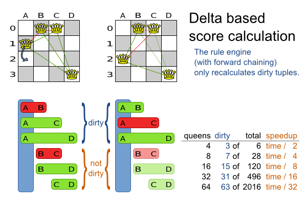
The speedup due to delta based score calculation is huge, because the speedup is relative to the size of your planning problem (your n). By using score rules, you get that speedup without writing any delta code.
If you know a certain constraint can never be broken, don't bother writing a score rule for it. For example in n queens, there is no "multipleQueensVertical" rule because a
Queen'scolumnnever changes and eachSolutionbuild puts eachQueenon a differentcolumn. This tends to give a huge performance gain, not just because the score function is faster, but mainly because mostSolverimplementations will spend less time evaluating unfeasible solutions.Be watchfull for score traps. A score trap is a state in which several moves need to be done to resolve or lower the weight of a single constraint occurrence. Some examples of score traps:
If you need 2 doctors at each table, but you're only moving 1 doctor at a time, then the solver has no insentive to move a doctor to a table with no doctors. Punish a table with no doctors more then a table with only 1 doctor in your score function.
If you only add the table as a cause of the ConstraintOccurrence and forget the jobType (which is doctor or politician), then the solver has no insentive to move a docter to table which is short of a doctor and a politician.
If you use tabu search, combine it with a
minimalAcceptedSelectionselector. Take some time to tweak the value ofminimalAcceptedSelection.Verify that your score calculation happens in the correct
Numbertype. If you're making the sum of integer values, don't let drools use Double's or your performance will hurt. TheSolverwill usually spend most of its execution time running the score function.Always remember that premature optimization is the root of all evil. Make sure your design is flexible enough to allow configuration based tweaking.
Currently, don't allow drools to backward chain instead of forward chain, so avoid query's. It kills delta based score calculation (so it kills scalibility).
Currently, don't allow drools to switch to MVEL mode, for performance.
For optimal performance, use at least java 1.6 and always use server mode (
java
        -server
). We have seen performance increases of 30% by switching from java 1.5 to 1.6 and 50% by turning on server mode.If you're doing performance tests, always remember that the JVM needs to warm up. First load your
Solverand do a short run, before you start benchmarking it.
In case you haven't figured it out yet: performance (and scalability) is very important for solving planning problems well. What good is a real-time freight routing solver that takes a day to find a feasible solution? Even small and innocent looking problems can hide an enormous problem size. For example, they probably still don't know the optimal solution of the traveling tournament problem for as little as 12 traveling teams.
In number of possible solutions for a planning problem can be mind blowing. For example:
4 queens has
256possible solutions (4 ^ 4) and 2 optimal solutions.5 queens has
3125possible solutions (5 ^ 5) and 1 optimal solution.8 queens has
16777216possible solutions (8 ^ 8) and 92 optimal solutions.64 queens has more than
10^115possible solutions (64 ^ 64).Most real-life planning problems have an incredible number of possible solutions and only 1 or a few optimal solutions.
For comparison: the minimal number of atoms in the known universe (10^80). As a planning problem gets bigger, the search space tends to blow up really fast. Adding only 1 extra planning entity or planning value can heavily multiply the running time of some algorithms.
An algorithm that checks every possible solution (even with pruning) can easily run for billions of years on a single real-life planning problem. What we really want is to find the best solution in the limited time at our disposal. Planning competitions (such as the International Timetabling Competition) show that local search variations (tabu search, simulated annealing, ...) usually perform best for real-world problems given real-world time limitations.
Drools Planner is the first framework to combine optimization algorithms (metaheuristics, ...) with score calculation by a rule engine such as Drools Expert. This combination turns out to be a very efficient, because:
A rule engine such as Drools Expert is great for calculating the score of a solution of a planning problem. It make it easy and scalable to add additional soft or hard constraints such as "a teacher shouldn't teach more then 7 hours a day". It does delta based score calculation without any extra code. However it tends to be not suited to use to actually find new solutions.
An optimization algorithm is great at finding new improving solutions for a planning problem, without necessarily brute-forcing every possibility. However it needs to know the score of a solution and offers no support in calculating that score efficiently.
Table 5.1. Optimization algorithms overview
| Algorithm | Scalable? | Optimal solution? | Needs little configuration? | Highly configurable? | Requires initialized solution? |
|---|---|---|---|---|---|
| Exact algorithms | |||||
| Brute force | 0/5 | 5/5 - Guaranteed | 5/5 | 0/5 | No |
| Branch and bound | 0/5 | 5/5 - Guaranteed | 4/5 | 1/5 | No |
| Construction heuristics | |||||
| First Fit | 5/5 | 1/5 - Stops after initialization | 5/5 | 1/5 | No |
| First Fit Decreasing | 5/5 | 2/5 - Stops after initialization | 4/5 | 2/5 | No |
| Best Fit | 5/5 | 2/5 - Stops after initialization | 4/5 | 2/5 | No |
| Best Fit Decreasing | 5/5 | 2/5 - Stops after initialization | 4/5 | 2/5 | No |
| Cheapest Insertion | 3/5 | 2/5 - Stops after initialization | 5/5 | 2/5 | No |
| Metaheuristics | |||||
| Local search | |||||
| Hill-climbing | 4/5 | 2/5 - Gets stuck in local optima | 3/5 | 3/5 | Yes |
| Tabu search | 4/5 | 4/5 | 3/5 | 5/5 | Yes |
| Simulated annealing | 4/5 | 4/5 | 2/5 | 5/5 | Yes |
| Evolutionary algorithms | |||||
| Evolutionary strategies | 4/5 | ?/5 | ?/5 | ?/5 | Yes |
| Genetic algorithms | 4/5 | ?/5 | ?/5 | ?/5 | Yes |
If you want to learn more about metaheuristics, read the free book Essentials of Metaheuristics or Clever Algorithms.
The best optimization algorithms configuration for your use case depends heavily on your use case. Nevertheless, this vanilla recipe will get you into the game with a pretty good configuration, probably much better than what you're used to.
Start with a quick configuration that involves little or no configuration and optimization code:
First Fit
Next, implement planning entity difficulty comparison and turn it into:
First Fit Decreasing
Next, implement moves and add tabu search behind it:
First Fit Decreasing
Tabu search (use property tabu or move tabu)
At this point the free lunch is over. The return on invested time lowers. The result is probably already more than good enough.
But you can do even better, at a lower return on invested time. Use the Benchmarker and try a couple of simulated annealing configurations:
First Fit Decreasing
Simulated annealing (try several starting temperatures)
And combine them with tabu search:
First Fit Decreasing
Simulated annealing (relatively long time)
Tabu search (relatively short time)
If you have time, continue experimenting even further. Blog about your experiments!
A Solver can use multiple optimization algorithms in sequence. Each
optimization algorithm is represented by a SolverPhase. There is never more than 1
SolverPhase solving at the same time.
Note
Some SolverPhase implementations can combine techniques from multiple optimization
algorithms, but they are still just 1 SolverPhase. For example: a local search
SolverPhase can do simulated annealing with property tabu.
Here's a configuration that runs 3 phases in sequence:
<solver>
  ...
  <constructionHeuristic>
    ... <!-- Phase 1: First Fit decreasing -->
  </constructionHeuristic>
  <localSearch>
    ... <!-- Phase 2: Simulated annealing -->
  </localSearch>
  <localSearch>
    ... <!-- Phase 3: Tabu search -->
  </localSearch>
</solver>
When the first phase terminates, the second phase starts, and so on. When the last phase terminates, the
Solver terminates.
Some phases (especially construction heuristics) will terminate automatically. Other phases (especially metaheuristics) will only terminate if the phase is configured to terminate:
<solver>
  ...
  <termination><!-- Solver termination -->
    <maximumSecondsSpend>90</maximumSecondsSpend>
  </termination>
  <localSearch>
    <termination><!-- Phase termination -->
      <maximumSecondsSpend>60</maximumSecondsSpend><!-- Give the next phase a chance to run too, before the Solver terminates -->
    </termination>
    ...
  </localSearch>
  <localSearch>
    ...
  </localSearch>
</solver>
If the Solver terminates (before the last phase terminates itself), the current phase is
terminated and all subsequent phases won't run.
Not all phases terminate automatically and sometimes you don't want to wait that long anyway. A
Solver can be terminated synchronously by up-front configuration or asynchronously from another
thread.
Especially metaheuristics phases will need to be told when to stop solving. This can be because of a number of reasons: the time is up, the perfect score has been reached, ... The only thing you can't depend on is on finding the optimal solution (unless you know the optimal score), because a metaheuristics algorithm generally doesn't know it when it finds the optimal solution. For real-life problems this doesn't turn out to be much of a problem, because finding the optimal solution could take billions of years, so you 'll want to terminate sooner anyway. The only thing that matters is finding the best solution in the available time.
For synchronous termination, configure a Termination on a Solver or a
SolverPhase when it needs to stop. You can implement your own Termination, but
the build-in implementations should suffice for most needs. Every Termination can calculate a
time gradient (needed for some optimization algorithms), which is a ratio between the time
already spend solving and the estimated entire solving time of the Solver or
SolverPhase.
Terminates when an amount of time has been reached:
    <termination>

        <maximumTimeMillisSpend>500</maximumTimeMillisSpend>

    </termination>
    <termination>

        <maximumSecondsSpend>10</maximumSecondsSpend>

    </termination>
    <termination>

        <maximumMinutesSpend>5</maximumMinutesSpend>

    </termination>
    <termination>

        <maximumHoursSpend>1</maximumHoursSpend>

    </termination>
Note
If you use this Termination, you will most likely sacrifice perfect reproducibility
(even with environmentMode REPRODUCIBLE) because of an available CPU time
difference:
The available CPU time influences the number of steps that can be taken, which might be a few more or less.
The
Terminationmight produce slightly different time gradient values, which will send time gradient based algorithms (such as simulated annealing) on a different path.
Terminates when a certain score has been reached. You can use this Termination if you
know the perfect score, for example for 4 queens:
    <termination>

        <scoreAttained>0</scoreAttained>

    </termination>
For a planning problem with hard and soft constraints, it could look like this:
    <termination>

        <scoreAttained>0hard/-5000soft</scoreAttained>

    </termination>
You can use this Termination to terminate once it reaches a feasible solution.
Terminates when an amount of steps has been reached:
    <termination>

        <maximumStepCount>100</maximumStepCount>

    </termination>
This Termination can only be used for a SolverPhase, not for the
Solver itself.
Terminates when the best score hasn't improved in a number of steps:
    <termination>

        <maximumUnimprovedStepCount>100</maximumUnimprovedStepCount>

    </termination>
If it hasn't improved recently, it's probably not going to improve soon anyway and it's not worth the effort to continue. We have observed that once a new best solution is found (even after a long time of no improvement on the best solution), the next few step tend to improve the best solution too.
Terminations can be combined, for example: terminate after 100 steps or if a score of 0 has been reached:
    <termination>

        <terminationCompositionStyle>OR</terminationCompositionStyle>

        <maximumStepCount>100</maximumStepCount>

        <scoreAttained>0</scoreAttained>

    </termination>
Alternatively you can use AND, for example: terminate after reaching a feasible score of at least -100 and no improvements in 5 steps:
    <termination>

        <terminationCompositionStyle>AND</terminationCompositionStyle>

        <maximumUnimprovedStepCount>5</maximumUnimprovedStepCount>

        <scoreAttained>-100</scoreAttained>

    </termination>
This example ensures it doesn't just terminate after finding a feasible solution, but also completes any obvious improvements on that solution before terminating.
Sometimes you 'll want to terminate a Solver early from another thread, for example because a user action or
a server restart. That cannot be configured by a Termination as it's impossible to predict when
and if it will occur. Therefor the Solver interface has these 2 thread-safe methods:
public interface Solver {


    // ...


    boolean terminateEarly();

    boolean isTerminateEarly();


}
If you call the terminateEarly() method from another thread, the
Solver will terminate at its earliest convenience and the solve() method
will return in the original Solver thread.
Between phases or before the first phase, you might want to execute a custom action on the
Solution to get a better score. Yet you'll still want to reuse the score calculation. For
example, to implement a custom construction heuristic without implementing an entire
SolverPhase.
Note
Most of the time, a custom construction heuristic is not worth the hassle. The supported constructions
heuristics are configurable (so you can tweak them with the Benchmarker),
Termination aware and support partially initialized solutions too.
Implement the CustomSolverPhaseCommand interface:
public interface CustomSolverPhaseCommand {

    void changeWorkingSolution(SolutionDirector solutionDirector);

}
For example:
public class ExaminationSolutionInitializer implements CustomSolverPhaseCommand {

    public void changeWorkingSolution(SolutionDirector solutionDirector) {
        Examination examination = (Examination) solutionDirector.getWorkingSolution();
        for (Exam exam : examination.getExamList()) {
            Score unscheduledScore = solutionDirector.calculateScoreFromWorkingMemory();
            ...
            for (Period period : examination.getPeriodList()) {
                exam.setPeriod(period)
                workingMemory.update(examHandle, exam);
                Score score = solutionDirector.calculateScoreFromWorkingMemory();
                ...
            }
            ...
        }
    }

}
Warning
Any change on the planning entities in a CustomSolverPhaseCommand must be told to the
WorkingMemory of solutionDirector.getWorkingMemory().
Warning
Do not change any of the planning facts in a CustomSolverPhaseCommand. That will corrupt
the Solver because any previous score or solution was for a different problem. If you want to
do that, see repeated planning and real-time planning instead.
And configure it like this:
<solver>
  ...
  <customSolverPhase>
    <customSolverPhaseCommandClass>org.drools.planner.examples.examination.solver.solution.initializer.ExaminationSolutionInitializer</customSolverPhaseCommandClass>
  </customSolverPhase>
  ... <!-- Other phases -->
</solver>
It's possible to configure multiple customSolverPhaseCommandClass instances, which will be
run in sequence.
Note
If the changes of a CustomSolverPhaseCommand don't result in a better score, the best
solution won't be changed (so effectively nothing will have changed for the next SolverPhase or
CustomSolverPhaseCommand). TODO: we might want to change this behaviour?
Note
If the Solver or SolverPhase wants to terminate while a
CustomSolverPhaseCommand is still running, it will wait to terminate until the
CustomSolverPhaseCommand is done.
Exact methods will always find the global optimum and recognize it too. That being said, they don't scale (not even beyond toy problems) and are therefor mostly useless.
The brute force algorithm creates and evaluates every possible solution.

Notice that it creates a search tree that explodes as the problem size increases. Brute force is mostly unusable for a real-world problem due to time limitations.
Branch and bound is an improvement over brute force, as it prunes away subsets of solutions which cannot have a better solution than the best solution already found at that point.

Notice that it (like brute force) creates a search tree that explodes (but less than brute force) as the problem size increases. Branch and bound is mostly unusable for a real-world problem due to time limitations.
It can determine a lower bound of problem. A lower bound is a score which is proven to be higher than the optimal score of a problem. So it gives an indication of the quality of any best solution found for that problem: the closer to best score is to the lower bound, the better.
A construction heuristic builds a pretty good initial solution in a finite length of time. Its solution isn't always feasible, but it finds it fast and metaheuristics can finish the job.
Construction heuristics terminate automatically, so there's usually no need to configure a
Termination on the construction heuristic phase specifically.
The First Fit algorithm cycles through all the planning entity (in default order), initializing 1 planning entity at a time. It assigns the planning entity to the best available planning value, taking the already initialized planning entities into account. It terminates when all planning entities have been initialized. It never changes a planning entity after it has been assigned.

Notice that it starts with putting Queen A into row 0 (and never moving it later), which
makes it impossible reach the optimal solution. Suffixing this construction heuristic with metaheurstics can
remedy that.
Configure this SolverPhase:
  <constructionHeuristic>
    <constructionHeuristicType>FIRST_FIT</constructionHeuristicType>
    <!-- Speedup that can be applied to most, but not all use cases: -->
    <!-- <constructionHeuristicPickEarlyType>FIRST_LAST_STEP_SCORE_EQUAL_OR_IMPROVING</constructionHeuristicPickEarlyType> -->
  </constructionHeuristic>
Note
The constructionHeuristicPickEarlyType of
FIRST_LAST_STEP_SCORE_EQUAL_OR_IMPROVING is a big speedup, which should be applied when
initializing a planning entity can only make the score lower or equal. So if:
There are no positive constraints.
There is no negative constraint that can stop been broken by adding a planning entity (except if another negative constraint gets broken which outweighs it the first negative constraint).
If that is not the case, then it can still be good to apply it in some cases, but not in most cases. Use
the Benchmarker to decide.
Like First Fit, but assigns the more difficult planning entities first, because they are
less likely to fit in the leftovers. So it sorts the planning entities on decreasing difficulty.
Requires the model to support planning entity difficulty comparison.

Note
One would expect that this algorithm always performs better than First Fit. That's not
always the case, but usually is.
Configure this SolverPhase:
  <constructionHeuristic>
    <constructionHeuristicType>FIRST_FIT_DECREASING</constructionHeuristicType>
    <!-- Speedup that can be applied to most, but not all use cases: -->
    <!-- <constructionHeuristicPickEarlyType>FIRST_LAST_STEP_SCORE_EQUAL_OR_IMPROVING</constructionHeuristicPickEarlyType> -->
</constructionHeuristic>Like First Fit, but uses the weaker planning values first, because the strong planning
values are more likely to be able to accomodate later planning entities. So it sorts the planning values on
increasing strength.
Requires the model to support planning value strength comparison.
Note
One would expect that this algorithm always performs better than First Fit. That's not
always the case.
Configure this SolverPhase:
  <constructionHeuristic>
    <constructionHeuristicType>BEST_FIT</constructionHeuristicType>
    <!-- Speedup that can be applied to most, but not all use cases: -->
    <!-- <constructionHeuristicPickEarlyType>FIRST_LAST_STEP_SCORE_EQUAL_OR_IMPROVING</constructionHeuristicPickEarlyType> -->
</constructionHeuristic>Combines First Fit Decreasing and Best Fit. So it sorts the planning
entities on decreasing difficulty and the planning values on increasing strength.
Requires the model to support planning entity difficulty comparison and planning value strength comparison.
Note
One would expect that this algorithm always performs better than First Fit,
First Fit Decreasing and Best Fit. That's not always the case.
Configure this SolverPhase:
  <constructionHeuristic>
    <constructionHeuristicType>BEST_FIT_DECREASING</constructionHeuristicType>
    <!-- Speedup that can be applied to most, but not all use cases: -->
    <!-- <constructionHeuristicPickEarlyType>FIRST_LAST_STEP_SCORE_EQUAL_OR_IMPROVING</constructionHeuristicPickEarlyType> -->
</constructionHeuristic>Local search starts from an initial solution and evolves that single solution into a mostly better and better solution. It uses a single search path of solutions, not a search tree. At each solution in this path it evaluates a number of moves on the solution and applies the most suitable move to take the step to the next solution. It does that for high number of iterations until its terminated (usually because its time has run out).
Local search acts a lot like a human planner: it uses a single search path and moves facts around to find a good feasible solution. Therefore it's pretty natural to implement.
Local search needs to start from an initialized solution, therefor it's recommended to configure a construction heuristic solver phase before it.
A move is the change from a solution A to a solution B. For example, below you can see a single move on the starting solution of 4 queens that moves a single queen to another row:
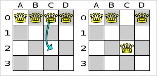
A move can have a small or large impact. In the above example, the move of queen C0 to C2 is a small move. Some moves are the same move type. These are some possibilities for move types in n queens:
Move a single queen to another row. This is a small move. For example, move queen C0 to C2.
Move all queens a number of rows down or up. This a big move.
Move a single queen to another column. This is a small move. For example, move queen C2 to A0 (placing it on top of queen A0).
Add a queen to the board at a certain row and column.
Remove a queen from the board.
Because we have decided that all queens will be on the board at all times and each queen has an appointed column (for performance reasons), only the first 2 move types are usable in our example. Furthermore, we 're only using the first move type in the example because we think it gives the best performance, but you are welcome to prove us wrong.
Each of your move types will be an implementation of the Move interface:
public interface Move {


    boolean isMoveDoable(EvaluationHandler evaluationHandler);


    Move createUndoMove(EvaluationHandler evaluationHandler);


    void doMove(EvaluationHandler evaluationHandler);


}
Let's take a look at the Move implementation for 4 queens which moves a queen to a
different row:
public class RowChangeMove implements Move {


    private Queen queen;

    private Row toRow;


    public RowChangeMove(Queen queen, Row toRow) {

        this.queen = queen;

        this.toRow = toRow;

    }


    // ... see below


}
An instance of RowChangeMove moves a queen from its current row to a different
row.
Drools Planner calls the doMove(WorkingMemory) method to do a move. The
Move implementation must notify the working memory of any changes it does on the solution
facts:
    public void doMove(WorkingMemory workingMemory) {

        FactHandle queenHandle = workingMemory.getFactHandle(queen);

        queen.setRow(toRow);

        workingMemory.update(queenHandle, queen); // after changes are made

    }
You need to call the workingMemory.update(FactHandle, Object) method after modifying the
fact. Note that you can alter multiple facts in a single move and effectively create a big move (also known as a
coarse-grained move).
Drools Planner automatically filters out non doable moves by calling the
isDoable(WorkingMemory) method on a move. A non doable move is:
A move that changes nothing on the current solution. For example, moving queen B0 to row 0 is not doable, because it is already there.
A move that is impossible to do on the current solution. For example, moving queen B0 to row 10 is not doable because it would move it outside the board limits.
In the n queens example, a move which moves the queen from its current row to the same row isn't doable:
    public boolean isMoveDoable(WorkingMemory workingMemory) {

        return !ObjectUtils.equals(queen.getRow(), toRow);

    }
Because we won't generate a move which can move a queen outside the board limits, we don't need to check it. A move that is currently not doable can become doable on a later solution.
Each move has an undo move: a move (usually of the same type) which does the exact opposite. In the above example the undo move of C0 to C2 would be the move C2 to C0. An undo move can be created from a move, but only before the move has been done on the current solution.
    public Move createUndoMove(WorkingMemory workingMemory) {

        return new RowChangeMove(queen, queen.getRow());

    }
Notice that if C0 would have already been moved to C2, the undo move would create the move C2 to C2, instead of the move C2 to C0.
The local search solver can do and undo a move more than once, even on different (successive) solutions.
A move must implement the equals() and hashcode() methods. 2 moves
which make the same change on a solution, must be equal.
    public boolean equals(Object o) {

        if (this == o) {

            return true;

        } else if (o instanceof RowChangeMove) {

            RowChangeMove other = (RowChangeMove) o;

            return new EqualsBuilder()

                    .append(queen, other.queen)

                    .append(toRow, other.toRow)

                    .isEquals();

        } else {

            return false;

        }

    }


    public int hashCode() {

        return new HashCodeBuilder()

                .append(queen)

                .append(toRow)

                .toHashCode();

    }
In the above example, the Queen class uses the default Object
equal() and hashcode() implementations. Notice that it checks if the other
move is an instance of the same move type. This is important because a move will be compared to a move with
another move type if you're using more then 1 move type.
It's also recommended to implement the toString() method as it allows you to read Drools
Planner's logging more easily:
    public String toString() {

        return queen + " => " + toRow;

    }
Now that we can make a single move, let's take a look at generating moves.
At each solution, local search will try all possible moves and pick the best move to change to the next solution. It's up to you to generate those moves. Let's take a look at all the possible moves on the starting solution of 4 queens:
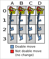
As you can see, not all the moves are doable. At the starting solution we have 12 doable moves (n *
(n - 1)), one of which will be move which changes the starting solution into the next solution. Notice
that the number of possible solutions is 256 (n ^ n), much more that the amount of doable
moves. Don't create a move to every possible solution. Instead use moves which can be sequentially combined to
reach every possible solution.
It's highly recommended that you verify all solutions are connected by your move set. This means that by combining a finite number of moves you can reach any solution from any solution. Otherwise you're already excluding solutions at the start. Especially if you're using only big moves, you should check it. Just because big moves outperform small moves in a short test run, it doesn't mean that they will outperform them in a long test run.
You can mix different move types. Usually you're better off preferring small (fine-grained) moves over big (course-grained) moves because the score delta calculation will pay off more. However, as the traveling tournament example proves, if you can remove a hard constraint by using a certain set of big moves, you can win performance and scalability. Try it yourself: run both the simple (small moves) and the smart (big moves) version of the traveling tournament example. The smart version evaluates a lot less unfeasible solutions, which enables it to outperform and outscale the simple version.
Move generation currently happens with a MoveFactory:
public class NQueensMoveFactory extends CachedMoveListMoveFactory {


    public List<Move> createMoveList(Solution solution) {

        NQueens nQueens = (NQueens) solution;

        List<Move> moveList = new ArrayList<Move>();

        for (Queen queen : nQueens.getQueenList()) {

            for (int y : nQueens.getRowList()) {

                moveList.add(new YChangeMove(queen, y));

            }

        }

        return moveList;

    }


}
But we might be making move generation part of the DRL's in the future.
A step is the winning move. The local search solver tries every move on the current solution and picks the best accepted move as the step:
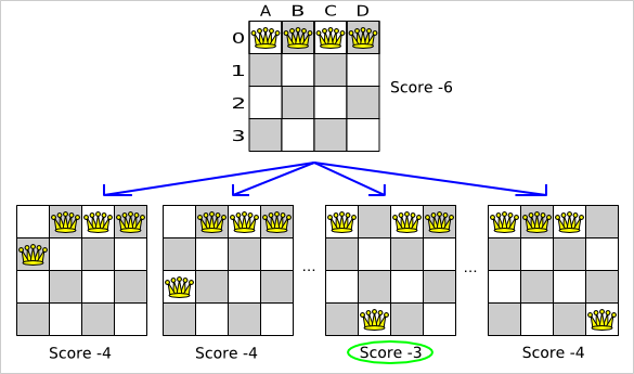
Because the move B0 to B3 has the highest score (-3), it is picked
as the next step. Notice that C0 to C3 (not shown) could also have been picked because it
also has the score -3. If multiple moves have the same highest score, one is picked randomly,
in this case B0 to B3.
The step is made and from that new solution, the local search solver tries all the possible moves again, to decide the next step after that. It continually does this in a loop, and we get something like this:
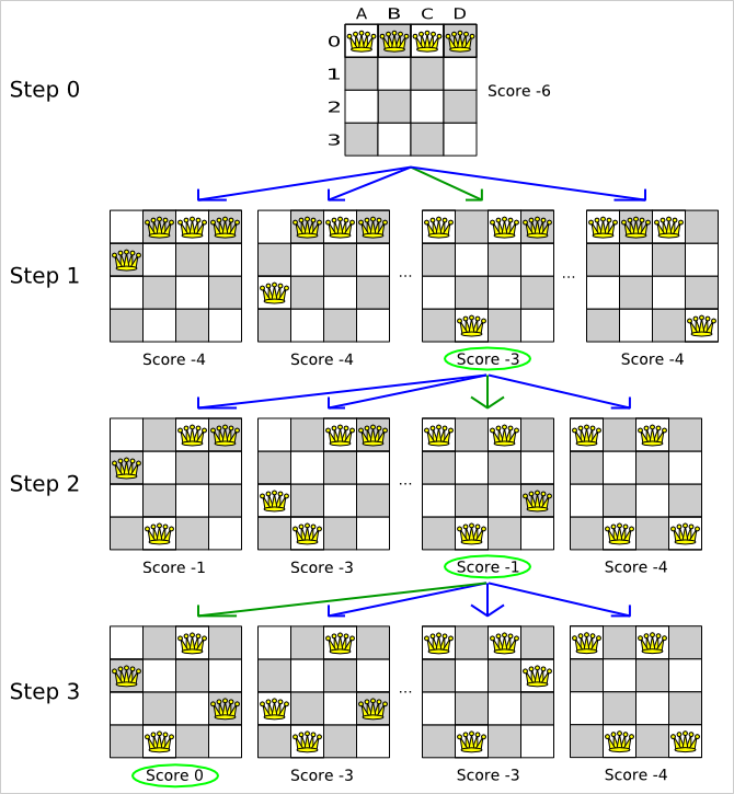
Notice that the local search solver doesn't use a search tree, but a search path. The search path is highlighted by the green arrows. At each step it tries all possible moves, but unless it's the step, it doesn't investigate that solution further. This is one of the reasons why local search is very scalable.
As you can see, the local search solver solves the 4 queens problem by starting with the starting solution and make the following steps sequentially:
B0 to B3
D0 to B2
A0 to B1
If we turn on DEBUG logging for the category org.drools.planner, then
those steps are shown into the log:
INFO  Solver started: time spend (0), score (-6), new best score (-6), random seed (0).
DEBUG     Step index (0), time spend (20), score (-3), new best score (-3), accepted move size (12) for picked step (col1@row0 => row3).
DEBUG     Step index (1), time spend (31), score (-1), new best score (-1), accepted move size (12) for picked step (col0@row0 => row1).
DEBUG     Step index (2), time spend (40), score (0), new best score (0), accepted move size (12) for picked step (col3@row0 => row2).
INFO  Phase local search finished: step total (3), time spend (41), best score (0).
INFO  Solved: time spend (41), best score (0), average calculate count per second (1780).
Notice that the logging uses the toString() method of our Move
implementation: col1@row0 => row3.
The local search solver solves the 4 queens problem in 3 steps, by evaluating only 37 possible solutions (3 steps with 12 moves each + 1 starting solution), which is only fraction of all 256 possible solutions. It solves 16 queens in 31 steps, by evaluating only 7441 out of 18446744073709551616 possible solutions. Note: with construction heurstistics it's even a lot more efficient.
A hill climber always takes improving moves. This may seem like a good thing, but it's not. It suffers from a number of problems:
It can get stuck in a local optimum. For example if it reaches a solution X with a score -1 and there is no improving move, it is forced to take a next step that leads to a solution Y with score -2, after that however, it's very real that it will pick the step back to solution X with score -1. It will then start looping between solution X and Y.
It can start walking in its own footsteps, picking the same next step at every step.
Of course Drools Planner implements better local searches, such as tabu search and simulated annealing which can avoid these problems. We recommend to never use a hill climber, unless you're absolutely sure there are no local optima in your planning problem.
The local search solver decides the next step with the aid of 3 configurable components:
A selector which selects (or generates) the possible moves of the current solution.
An acceptor which filters out unacceptable moves. It can also weigh a move it accepts.
A forager which gathers all accepted moves and picks the next step from them.
In the above example the selector generated the moves shown with the blue lines, the acceptor accepted all of them and the forager picked the move B0 to B3.
If we turn on TRACE logging for the category org.drools.planner, then
the decision making is shown in the log:
INFO  Solver started: time spend (0), score (-6), new best score (-6), random seed (0).
TRACE         Ignoring not doable move (col0@row0 => row0).
TRACE         Move score (-4), accepted (true) for move (col0@row0 => row1).
TRACE         Move score (-4), accepted (true) for move (col0@row0 => row2).
TRACE         Move score (-4), accepted (true) for move (col0@row0 => row3).
...
TRACE         Move score (-3), accepted (true) for move (col1@row0 => row3).
...
TRACE         Move score (-3), accepted (true) for move (col2@row0 => row3).
...
TRACE         Move score (-4), accepted (true) for move (col3@row0 => row3).
DEBUG     Step index (0), time spend (6), score (-3), new best score (-3), accepted move size (12) for picked step (col1@row0 => row3).
...
A selector is currently based on a MoveFactory.
  <selector>

    <moveFactoryClass>org.drools.planner.examples.nqueens.solver.NQueensMoveFactory</moveFactoryClass>

  </selector>
You're not obligated to generate the same set of moves at each step. It's generally a good idea to use several selectors, mixing fine grained moves and course grained moves:
  <selector>

    <selector>

      <moveFactoryClass>org.drools.planner.examples.nurserostering.solver.move.factory.EmployeeChangeMoveFactory</moveFactoryClass>

    </selector>

    <selector>

      <moveFactoryClass>org.drools.planner.examples.nurserostering.solver.move.factory.ShiftAssignmentSwitchMoveFactory</moveFactoryClass>

    </selector>

    <selector>

      <moveFactoryClass>org.drools.planner.examples.nurserostering.solver.move.factory.ShiftAssignmentPillarPartSwitchMoveFactory</moveFactoryClass>

    </selector>

  </selector>
An acceptor is used (together with a forager) to active tabu search, simulated annealing, great deluge, ... For each move it checks whether it is accepted or not.
You can implement your own Acceptor, although the build-in acceptors should suffice for
most needs. You can also combine multiple acceptors.
When tabu search takes steps it creates tabu's. It does not accept a move as the next step if that move breaks tabu. Drools Planner implements several tabu types:
Solution tabu makes recently visited solutions tabu. It does not accept a move that leads to one of those solutions. If you can spare the memory, don't be cheap on the tabu size.
    <acceptor>

        <solutionTabuSize>1000</solutionTabuSize>

    </acceptor>
Move tabu makes recent steps tabu. It does not accept a move equal to one of those steps.
    <acceptor>

        <moveTabuSize>7</moveTabuSize>

    </acceptor>
Undo move tabu makes the undo move of recent steps tabu.
    <acceptor>

        <undoMoveTabuSize>7</undoMoveTabuSize>

    </acceptor>
Property tabu makes a property of recent steps tabu. For example, it can make the queen tabu, so that a recently moved queen can't be moved.
    <acceptor>

        <propertyTabuSize>5</propertyTabuSize>

    </acceptor>
To use property tabu, your moves must implement the
TabuPropertyEnabledinterface, for example:public class YChangeMove implements Move, TabuPropertyEnabled {
private Queen queen;
private Row toRow;
// ...
public List<? extends Object> getTabuPropertyList() {
return Collections.singletonList(queen);
}
}You can also make multiple properties tabu (with OR or AND semantics):
    public List<? extends Object> getTabuPropertyList() {

        // tabu with other moves that contain the same leftExam OR the same rightExam

        return Arrays.asList(leftExam, rightExam);

    }
public List<? extends Object> getTabuPropertyList() {
// tabu with other moves that contain the same exam AND the same toPeriod (but not necessary the same toRoom)
return Collections.singletonList(Arrays.asList(exam, toPeriod));
}
You can even combine tabu types:
    <acceptor>

        <solutionTabuSize>1000</solutionTabuSize>

        <moveTabuSize>7</moveTabuSize>

    </acceptor>
If you pick a too small tabu size, your solver can still get stuck in a local optimum. On the other hand, with the exception of solution tabu, if you pick a too large tabu size, your solver can get stuck by bouncing of the walls. Use the benchmarker to fine tweak your configuration. Experiments teach us that it is generally best to use a prime number for the move tabu, undo move tabu or property tabu size.
A tabu search acceptor should be combined with a high or no subset selection.
Simulated annealing does not always pick the move with the highest score, neither does it evaluate many
moves per step. At least at first. Instead, it gives unimproving moves also a chance to be picked, depending on
its score and the time gradient of the Termination. In the end, it gradually turns into a
hill climber, only accepting improving moves.
In many use cases, simulated annealing surpasses tabu search. By changing a few lines of configuration, you can easily switch from tabu search to simulated annealing and back.
Start with a simulatedAnnealingStartingTemperature set to the maximum score delta a
single move can cause. Use the Benchmarker to tweak the value.
    <acceptor>

      <simulatedAnnealingStartingTemperature>2hard/100soft</simulatedAnnealingStartingTemperature>

    </acceptor>

    <forager>

        <minimalAcceptedSelection>4</minimalAcceptedSelection>

    </forager>
A simulated annealing acceptor should be combined with a low subset selection. The classic algorithm uses
a minimalAcceptedSelection of 1, but usually 4 performs
better.
You can even combine it with a tabu acceptor at the same time. Use a lower tabu size than in a pure tabu search configuration.
    <acceptor>

      <simulatedAnnealingStartingTemperature>10.0</simulatedAnnealingStartingTemperature>

      <propertyTabuSize>5</propertyTabuSize>

    </acceptor>

    <forager>

        <minimalAcceptedSelection>4</minimalAcceptedSelection>

    </forager>
This differs from phasing, another powerful technique, where first simulated annealing is used, followed by tabu search.
A forager gathers all accepted moves and picks the move which is the next step. Normally it picks the accepted move with the highest score. If several accepted moves have the highest score, one is picked randomly.
You can implement your own Forager, although the build-in forager should suffice for most
needs.
When there are many possible moves, it becomes inefficient to evaluate all of them at every step. To evaluate only a random subset of all the moves, use:
An
minimalAcceptedSelectioninteger, which specifies how many accepted moves should have be evaluated during each step. By default it is positive infinity, so all accepted moves are evaluated at every step.<forager>
<minimalAcceptedSelection>1000</minimalAcceptedSelection>
</forager>
Unlike the n queens problem, real world problems require the use of subset selection. Start from an
minimalAcceptedSelection that takes a step in less then 2 seconds. Turn on INFO logging to
see the step times. Use the Benchmarker to tweak the value.
A forager can pick a move early during a step, ignoring subsequent selected moves. There are 3 pick early types:
NEVER: A move is never picked early: all accepted moves are evaluated that the selection allows. This is the default.<forager>
<pickEarlyType>NEVER</pickEarlyType>
</forager>
FIRST_BEST_SCORE_IMPROVING: Pick the first accepted move that improves the best score. If none improve the best score, it behaves exactly like the pickEarlyType NEVER.<forager>
<pickEarlyType>FIRST_BEST_SCORE_IMPROVING</pickEarlyType>
</forager>
FIRST_LAST_STEP_SCORE_IMPROVING: Pick the first accepted move that improves the last step score. If none improve the last step score, it behaves exactly like the pickEarlyType NEVER.<forager>
<pickEarlyType>FIRST_LAST_STEP_SCORE_IMPROVING</pickEarlyType>
</forager>
Because the current solution can degrade (especially in tabu search and simulated annealing), the
Solver remembers the best solution it has encountered through the entire search path. Each time
the current solution is better than the last best solution, the current solution is cloned and referenced as the new
best solution.
You can listen to solver events, including when the best solution changes during solving, by adding a
SolverEventListener to the Solver:
public interface Solver {
// ...
void addEventListener(SolverEventListener eventListener);
void removeEventListener(SolverEventListener eventListener);
}
It is easy to plug in a custom Selector, Acceptor,
Forager or Termination by extending the abstract class and also the config
class.
For example, to use a custom Selector, extend the AbstractSelector class
(see AllMovesOfOneExamSelector), extend the SelectorConfig class (see
AllMovesOfOneExamSelectorConfig) and configure it in the configuration XML:
<selector class="org.drools.planner.examples.examination.solver.selector.AllMovesOfOneExamSelectorConfig"/>
If you build a better implementation that's not domain specific, consider adding it as a patch in our issue tracker and we'll take it along in future refactors and optimize it.
Drools Planner supports several solver types, but you're probably wondering which is the best one? Although some solver types generally perform better then others, it really depends on your problem domain. Most solver types also have settings which can be tweaked. Those settings can influence the results of a solver a lot, although most settings perform pretty good out-of-the-box.
Luckily, Drools Planner includes a benchmarker, which allows you to play out different solver types and different settings against each other, so you can pick the best configuration for your problem domain.
The Benchmarker is current in the drools-planner-core modules, but it requires an extra dependency on the JFreeChart library.
If you use maven, add a dependency in your pom.xml file:
<dependency>
<groupId>jfree</groupId>
<artifactId>jfreechart</artifactId>
<version>1.0.13</version>
</dependency>This is similar for gradle, ivy and buildr.
If you use ANT, you've probably already copied the required jars from the download zip's
binaries directory.
You can build a Benchmarker instance with theXmlSolverBenchmarker.
Configure it with a benchmarker configuration xml file:
XmlSolverBenchmarker benchmarker = new XmlSolverBenchmarker();
benchmarker.configure("/org/drools/planner/examples/nqueens/benchmark/nqueensSolverBenchmarkConfig.xml");
benchmarker.benchmark();
benchmarker.writeResults(resultFile);
A basic benchmarker configuration file looks something like this:
<?xml version="1.0" encoding="UTF-8"?>
<solverBenchmarkSuite>
<benchmarkDirectory>local/data/nqueens</benchmarkDirectory>
<solverStatisticType>BEST_SOLUTION_CHANGED</solverStatisticType>
<warmUpSecondsSpend>30</warmUpSecondsSpend>
<inheritedSolverBenchmark>
<unsolvedSolutionFile>data/nqueens/unsolved/unsolvedNQueens32.xml</unsolvedSolutionFile>
<unsolvedSolutionFile>data/nqueens/unsolved/unsolvedNQueens64.xml</unsolvedSolutionFile>
<solver>
<solutionClass>org.drools.planner.examples.nqueens.domain.NQueens</solutionClass>
<planningEntityClass>org.drools.planner.examples.nqueens.domain.Queen</planningEntityClass>
<scoreDrl>/org/drools/planner/examples/nqueens/solver/nQueensScoreRules.drl</scoreDrl>
<scoreDefinition>
<scoreDefinitionType>SIMPLE</scoreDefinitionType>
</scoreDefinition>
<termination>
<maximumSecondsSpend>20</maximumSecondsSpend>
</termination>
<constructionHeuristic>
<constructionHeuristicType>FIRST_FIT_DECREASING</constructionHeuristicType>
<constructionHeuristicPickEarlyType>FIRST_LAST_STEP_SCORE_EQUAL_OR_IMPROVING</constructionHeuristicPickEarlyType>
</constructionHeuristic>
</solver>
</inheritedSolverBenchmark>
<solverBenchmark>
<name>Solution tabu</name>
<solver>
<localSearch>
<selector>
<moveFactoryClass>org.drools.planner.examples.nqueens.solver.move.factory.RowChangeMoveFactory</moveFactoryClass>
</selector>
<acceptor>
<solutionTabuSize>1000</solutionTabuSize>
</acceptor>
    <forager>

        <pickEarlyType>NEVER</pickEarlyType>

    </forager>
</localSearch>
</solver>
</solverBenchmark>
<solverBenchmark>
<name>Move tabu</name>
<solver>
<localSearch>
<selector>
<moveFactoryClass>org.drools.planner.examples.nqueens.solver.move.factory.RowChangeMoveFactory</moveFactoryClass>
</selector>
<acceptor>
<moveTabuSize>5</moveTabuSize>
</acceptor>
<forager>
<pickEarlyType>NEVER</pickEarlyType>
</forager>
</localSearch>
</solver>
</solverBenchmark>
<solverBenchmark>
<name>Property tabu</name>
<solver>
<localSearch>
<selector>
<moveFactoryClass>org.drools.planner.examples.nqueens.solver.move.factory.RowChangeMoveFactory</moveFactoryClass>
</selector>
<acceptor>
<propertyTabuSize>5</propertyTabuSize>
</acceptor>
<forager>
<pickEarlyType>NEVER</pickEarlyType>
</forager>
</localSearch>
</solver>
</solverBenchmark>
</solverBenchmarkSuite>
This benchmarker will try 3 configurations (1 solution tabu, 1 move tabu and 1 property tabu) on 2 data sets (32 and 64 queens), so it will run 6 solvers.
Every solverBenchmark entity contains a solver configuration (for example a local search
solver) and one or more unsolvedSolutionFile entities. It will run the solver configuration on
each of those unsolved solution files. A name is optional and generated if absent.
The common part of multiple solverBenchmark entities can be extracted to the
inheritedSolverBenchmark entity, but that can still be overwritten per
solverBenchmark entity. Note that inherited solver phases such as
<constructionHeuristic> or <localSearch> are not overwritten but
instead are added to the head of the solver phases list.
You need to specify a benchmarkDirectory (relative to the working directory). The best
solution of each solver run and a handy overview HTML webpage will be written in that directory.
Without a warmup, the results of the first (or first few) benchmarks are not reliable, because they will have lost CPU time on hotspot JIT compilation (and possibly DRL compilation too).
The avoid that distortion, the benchmarker can run some of the benchmarks for a specified amount of time, before running the real benchmarks. Generally, a warm up of 30 seconds suffices:
<solverBenchmarkSuite>
  ...
  <warmUpSecondsSpend>30</warmUpSecondsSpend>
  ...
</solverBenchmarkSuite>
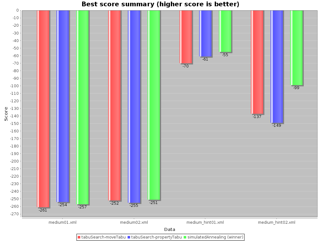
The benchmarker supports outputting statistics as graphs and CSV (comma separated values) files to the
benchmarkDirectory.
To configure graph and CSV output of a statistic, just add a solverStatisticType
line:
<solverBenchmarkSuite>

  <benchmarkDirectory>local/data/nqueens/solved</benchmarkDirectory>

  <solverStatisticType>BEST_SOLUTION_CHANGED</solverStatisticType>

  ...

</solverBenchmarkSuite>
Multiple solverStatisticType entries are allowed. Some statistic types might influence
performance noticeably. The following types are are supported:
To see how the best score evolves over time, add BEST_SOLUTION_CHANGED as a
solverStatisticType.
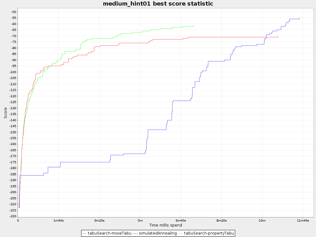
Note
Don't be fooled by the simulated annealing line in this graph. If you give simulated annealing only 5 minutes, it might still be better than 5 minutes of tabu search. That's because this simulated annealing implementation automatically determines it's velocity based on the amount of time that can be spend. On the other hand, for the tabu search, what you see is what you'd get.
To see how fast the scores are calculated, add CALCULATE_COUNT_PER_SECOND as a
solverStatisticType.
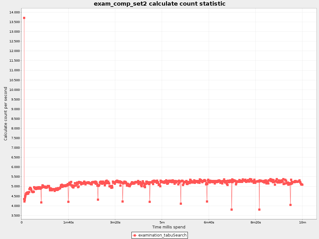
Note
The initial high calculate count is typical during solution initialization. In this example, it's far easier to calculate the score of a solution if only a handful exams have been added, in contrast to all of them. After those few seconds of initialization, the calculate count is relatively stable, apart from an occasional stop-the-world garbage collector disruption.
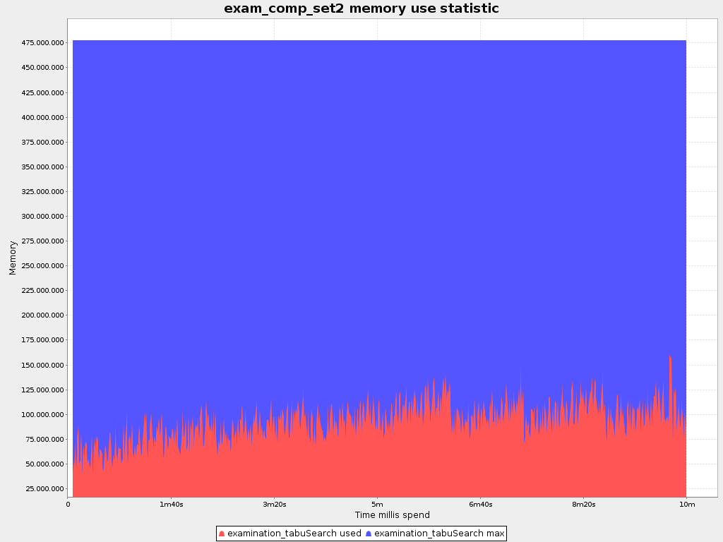
The world constantly changes. The planning facts used to create a solution, might change before or during the execution of that solution. There are 3 types of situations:
Unforeseen fact changes: For example: an employee assigned to a shift calls in sick, an airplane scheduled to take off has a technical delay, one of the machines or vehicles break down, ... Use backup planning.
Unknown long term future facts: For example: The hospital admissions for the next 2 weeks are reliable, but those for week 3 and 4 are less reliable and for week 5 and beyond are not worth planning yet. Use continuous planning.
Constantly changing planning facts: Use real-time planning.
Waiting to start planning - to lower the risk of planning facts changing - usually isn't a good way to deal with that. More CPU time means a better planning solution. An incomplete plan is better then no plan.
Luckily, the Drools Planner algorithms support planning a solution that's already (partially) planned, known as repeated planning.
Backup planning is the technique of adding extra score constraints to create space in the planning for when things go wrong. That creates a backup plan in the plan. For example: try to assign an employee as the spare employee (1 for every 10 shifts at the same time), keep 1 hospital bed open in each department, ...
Then, when things go wrong (one of the employees calls in sick), change the planning facts on the original solution (delete the sick employee leave his/her shifts unassigned) and just restart the planning, starting from that solution, which has a different score now. The construction heuristics will fill in the newly created gaps (probably with the spare employee) and the metaheuristics will even improve it further.
Continuous planning is the technique of planning one or more upcoming planning windows at the same time and repeating that process every week (or every day). Because time infinite, there are an infinite future windows, so planning all future windows is impossible. Instead we plan only a number of upcoming planning windows.
Past planning windows are immutable. The first upcoming planning window is considered stable (unlikely to change), while later upcoming planning windows are considered draft (likely to change during the next planning effort). Distant future planning windows are not planned at all.
Past planning windows have locked planning entities: the planning entities can no longer be changed (they are locked in place), but some of them are still needed in the working memory, as they might affect some of the score constraints that apply on the upcoming planning entities. For example: when an employee should not work more than 5 days in a row, he shouldn't work today and tomorrow if he worked the past 4 days already.
Sometimes some planning entities are semi-locked: they can be changed, but occur a certain score penalty if they differ from their original place. For example: avoid rescheduling hospital beds less than 2 days before the patient arrives (unless it's really worth it), avoid changing the airplane gate (or worse, the terminal) during the 2 hours before boarding, ...
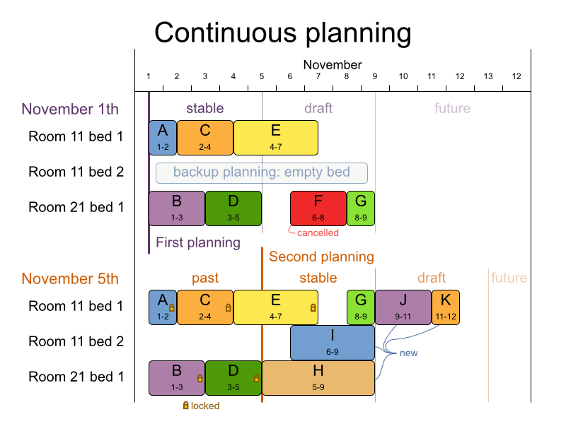
Notice the difference between the original planning of November 1th and the new planning of November 5th: some planning facts (F, H, I, J, K) changed, which results in unrelated planning entities (G) changing too.
To do real-time planning, first combine backup planning and continuous planning with short planning windows to
lower the burden of real-time planning. Don't configure any Termination, just terminate early
when you need the results or subscribe to the BestSolutionChangedEvent (the latter doesn't
guarantee yet that every ProblemFactChange has been processed already).
While the Solver is solving, an outside event might want to change one of the problem
facts, for example an airplane is delayed and needs the runway at a later time. Do not change the problem fact
instances used by the Solver while it is solving, as that will corrupt it. Instead, add a
ProblemFactChange to the Solver which it will execute as soon as the timing is
right.
public interface Solver {

   ...

   boolean addProblemFactChange(ProblemFactChange problemFactChange);

   ...

}
public interface ProblemFactChange {
void doChange(SolutionDirector solutionDirector);
}Here's an example:
    public void deleteComputer(final CloudComputer cloudComputer) {
        solver.addProblemFactChange(new ProblemFactChange() {
            public void doChange(SolutionDirector solutionDirector) {
                CloudBalance cloudBalance = (CloudBalance) solutionDirector.getWorkingSolution();
                WorkingMemory workingMemory = solutionDirector.getWorkingMemory();
                // First remove the planning fact from all planning entities that use it
                for (CloudProcessAssignment cloudProcessAssignment : cloudBalance.getCloudProcessAssignmentList()) {
                    if (ObjectUtils.equals(cloudProcessAssignment.getCloudComputer(), cloudComputer)) {
                        FactHandle cloudProcessAssignmentHandle = workingMemory.getFactHandle(cloudProcessAssignment);
                        cloudProcessAssignment.setCloudComputer(null);
                        workingMemory.retract(cloudProcessAssignmentHandle);
                    }
                }
                // Next remove it the planning fact itself
                for (Iterator<CloudComputer> it = cloudBalance.getCloudComputerList().iterator(); it.hasNext(); ) {
                    CloudComputer workingCloudComputer = it.next();
                    if (ObjectUtils.equals(workingCloudComputer, cloudComputer)) {
                        FactHandle cloudComputerHandle = workingMemory.getFactHandle(workingCloudComputer);
                        workingMemory.retract(cloudComputerHandle);
                        it.remove(); // remove from list
                        break;
                    }
                }
            }
        });
    }
Warning
Any change on the problem facts or planning entities in a ProblemFactChange must be done
on the instances of the Solution of
solutionDirector.getWorkingSolution().
Warning
Any change on the problem facts or planning entities in a ProblemFactChange must be told
to the WorkingMemory of solutionDirector.getWorkingMemory().
Note
Many types of changes can leave a planning entity uninitialized, resulting in a partially initialized
solution. That's fine, as long as the first solver phase can handle it. All construction heuristics solver phases
can handle that, so it's recommended to configure such a SolverPhase as the first phase.
In essence, the Solver will stop, run the ProblemFactChange and restart.
Each SolverPhase will be run again. Each configured Termination (except
terminateEarly) will reset.