(name, value, timestamp, ttl)
Overview
This page provides a brief summary of the different database technologies that have been take into consideration as RHQ's next generation metrics storage solution. The information provided for each technology is not intended to be exhaustive. The intent is to compare and contrast key features, better understand strengths and weaknesses, and ultimately become more informed about what is the best fit for our needs. The last section on this page provides a summary of key features and recommendation of which database should be used.
|
Database |
Performance |
Scalability |
Management |
Clustering Architecture |
Data Model |
Fault Tolerance |
Consistency |
Replication |
Data Processing |
Ad hoc queries |
|
Infinispan |
fast reads |
incremental |
JMX |
P2P, dynamo style |
key/value, java.util.Map |
highly available |
tunable consistency |
configurable per cache |
MapReduce, Distributed Execution Framework |
none |
|
Cassandra |
constant time writes |
incremental |
JMX |
P2P, dynamo style |
key/value, column-oriented (BigTable) |
highly available |
tunable consistency |
configurable per schema |
external Hadoop integration |
limited via CQL |
|
MongoDB |
fast reads |
sharding + replica sets |
Built-in commands, external utilities |
Master/Slave |
document-oriented |
Provides automated failover via replica sets |
strong consistency |
fully replicated |
MapReduce, Aggregation framework |
excellent support |
|
HBase |
fast scans |
sharding |
JMX |
Master/Slave, HDFS |
key/value, column-oriented (BigTable) |
Provides automated region server fail over |
strong consistency |
fully replicated |
Hadoop MapReduce |
external support via hive |
Infinispan
Infinispan is a distributed key value store and compute grid that is a JBoss project developed in-house.
Performance
Both high performance reads as well as writes are possible with Infinispan. Infinispan is extremely flexible. Some caches can be configured to be in-memory only while others can be configured to use a persistent store. The persistent stores that are used pluggable. Caches can be configured to use a shared persistent store or separate ones. Reads and writes can be done asynchronously allowing for greater throughput.
Scalability
Infinispan is highly scalable. It uses a P2P model where any node can service a read or a write request. Nodes can be added to the cluster at any time. It should be noted that adding a node can be an expensive operation as it may result in redistributing data around the grid; consequently, it is best to do this during a maintenance period. The important thing to take away is that it is possible achieve faster writes without sacrificing on read performance and vice versa.
Administration and Management
One of the biggest selling points of Infinispan as a possible solution is that it is a JBoss project that is fully supported by Red Hat. There is already an existing Infinispan plugin for RHQ.
Clustering Architecture
Infinispan has a P2P architecture with no single point of failure. Any node can service a read or write request. JGroups is used at the comm layer.
Data Model
Infinispan is a distributed cache which means at its core we are dealing with java.util.Map. The cache and map APIs, with their level of granularity, do not lend themselves well to managing time series data. With time series data, whether it is numeric data, call time data, or events, we are essentially dealing with continuous streams of data. We take samples or slices of those streams to generate graphs and charts and to calculate aggregates. We faced some obstacles around querying and indexing.
Let's consider fetching some range of metric data points. Suppose there are N data points. On the one hand, we can store one cache entry per data point. Storing the data is easy. It is just a simple cache write for each data point, and no reads are required to store the entry. Fetching the data however is problematic. Doing N cache reads would be very inefficient in most situations except N is very small. Aside from the size of N, this presupposes that we already know the key for each cache entry. You need to know the key in order to read an entry from a cache. Storing a cache entry per data point is not a very good approach. Now let's consider the other end of the spectrum where we store all data points in a single cache entry. The advantage to this approach is that we can fetch all the data points for the query in a single cache read. This strategy however is much more inefficient that storing a single entry per data point. For every data point that we insert, we have to first read the entry from the cache. As the number of data points grow, the cache entry will become prohibitively large.
A better approach than the ones previously discussed is to store a group of data points in each cache entry. For raw data we can group the data points by the hour. This would yield at most 120 data points per entry. Suppose that the query spans a time period of four hours. This would translate into four cache reads. This solution helps to minimize the number of reads for a query as well as provides a basic paging mechanism. Implementing this presents a challenge. In order to sustain high throughput for writing metric data, we want to avoid having to do any reads for a write. We want to avoid having to first read the hourly entry, add the raw data to, and the write the entry back into the cache. When storing raw metric data, we can easily determine the group to which it belongs by rounding down to the top of the hour. This will give us the cache entry key which would consist of the metric schedule id and the hour timestamp. To avoid read-on-writes, we can utilize Infinispan's Distributed Executor Framework. We write the raw data into a staging cache and submit a background task to add the raw data to the hourly entry. This approach seemed to work fairly well for our initial prototyping efforts. There is one catch though. It requires us to know the key or keys in advance.
For queries where we do not know the keys in advance, we have to rely on the Distributed Executor Framework or MapReduce. Aside from having to essentially write a Java program for a query, a potentially bigger problem is the lack of support for any kind of paging. The output of a MapReduce job is a single object does not provide an efficient way to page through or stream results.
The other problem we ran into was how to create efficient indexes. We need indexes in a number of places. For example, we need indexes so that we can quickly determine what metric data needs to be aggregated. Infinispan provides AtomicHashMap which we might have been able to use to build reasonably efficient data structures. We opted against that though because it can only be used with a transactional cache. We want to avoid the overhead of transactions at all costs. The approach we went with was to use dedicated caches as our indexes. There are two main benefits. It allows us to avoid locking and transactions, and it also enables us to avoid doing read-before-write. The big drawback is that we have to rely on MapReduce or the Distributed Executor Framework to search the index cache.
Fault Tolerance
Infinispan is a highly available data store. It is very resilient to failure. There is no single point of failure with its P2P architecture. Replication plays a major role here is role. It is discussed subsequently in its own section. I am not sure what if any type of recovery options currently exist for situations like a failed write to a node during replication.
Consistency
Consistency is tunable within Infinispan. A cache can be configured to use <async> communication which means when data is propagated to other nodes, the sender does not wait for responses from those nodes.
Replication
Replication is configurable on a per cache basis. There is a configuration option to specify the number of copies of data that should exist in the cluster.
Data Processing
MapReduce, Distributed Execution Framework
HBase
HBase is a column-oriented database that follows the BigTable design for its data model. HBase is sometimes referred to as the Hadoop database because it runs on HDFS, the Hadoop Distributed File System. HBase has not been actively considered for a solution; however, I wanted to include it in this discussion due to the ever growing mind share Hadoop has. We need to look at some the architectural details of HDFS and HBase in order to understand why HBase is not a good fit for RHQ.
HDFS has a master/slave architecture. There is a single name node that is the master server. It manages the file system namespace as well as client access. There is a secondary name node whose purpose is to provide periodic checkpoints on the name node. It downloads the current name node image and edits log files. A new image is created and uploaded back to the name node. The secondary name node does not provide failover; consequently, the name node is a single point of failure in HDFS. For production use both the name node and secondary name nodes should run on separate machines. Then there are data node which manage the content stored on them. There can be any number of data nodes. Files in HDFS are split into blocks that are spread across the data nodes.
An HBase cluster consists of a master server and multiple region servers. The master server monitors all region servers in the cluster and handles all meta data changes. It also takes care of splitting or balancing data across the cluster. A region server is responsible for handling client requests, e.g., get, put, delete, etc. The master server typically runs on the same machine as the HDFS name node, and region servers usually run on the same machines that HDFS data nodes run on. Because clients talk directly to region servers, the cluster can continue to function if the master server goes down, albeit in a limited capacity since the master controls critical functions like region server failover and data splitting. It is possible to run multiple master nodes to provide failover.
HBase necessitates a lot of moving parts with multiple failure points, all of which increase the complexity in terms of management. Then if you throw in Hadoop MapReduce for data processing, we have even more components to run and manage with the job tracker and task tracker. Simply put, there are other available solutions with substantially lower management complexity that allow us to meet our data processing needs.
Cassandra
Cassandra is a key/value store or column-oriented database. Its data model is similar to the one described in the BigTable paper. It follows a Dynamo-based architecture for consistency and availability.
Performance
Writes in Cassandra are extremely fast - faster than reads and much faster than other databases, relational or otherwise. There is no random IO involved with writes. Two things happen with a write. The operation is appended to the commit log on disk, and the MemTable, the in-memory data structure for a column family, is updated. Reads are fast provided the data is in memory. As with other databases the performance hit comes when Cassandra has to go to disk. The on-disk representation of a MemTable is called an SSTable. Multiple SSTables may exist for a given MemTable or column family. Each SSTable is stored in its own file on disk. For a read, it is possible that data may exist entirely in the MemTable, or it may exist entirely on disk in one or more SSTables, or it may exist in some combination of the two.
Cassandra's key and row caching can further improve read performance. The key cache stores the location of keys in memory whereas the row cache stores the entire contents of a row in memory. A row cache hit will altogether eliminate going to disk, and a key cache hit will eliminate a disk seek.
Scalability
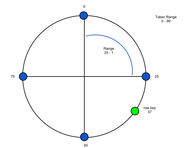
Cassandra provides linear scalability. When additional capacity is needed, you simply add more nodes to the cluster. A node can auto bootstrap itself such it that learns the cluster topology, discovering other nodes in the cluster, and it obtain data for which it is responsible from other nodes in the cluster. Like Infinispan, Cassandra uses consistent hashing. The cluster forms a token ring, and each node is responsible for an equal portion of the ring. When nodes are added or removed from the cluster, tokens (or token ranges) for each node should be recalculated to keep the ring balanced. When tokens are recalculated, the portion of the ring for which node is responsible may change. This may result in additional data being moved around the cluster. There is an effort underway to add support for virtual nodes. Virtual nodes will help simplify cluster management operations like adding/remove nodes and help further improve load distribution. This work is being tracked under CASSANDRA-4119.
Administration and Management
One of the big selling points of Cassandra is the minimal administration involved. There is only a single process per node and a single configuration file, cassandra.yaml. Cassandra was designed with high availability and fault tolerance in mind. This in turn simplifies management. Let me illustrate with a couple of examples. Cassandra nodes can be configured to use a snitch. A snitch determines the overall network topology of the cluster and uses that information to route inter-node requests as efficiently as possible. There are a number of different types of snitches that are suited for different deployment scenarios. All snitches monitor read latency and when possible route traffic away from poorly performing nodes.
Another feature that simplifies management is hinted handoffs. If there is a write and the replica node for the key is down, Cassandra will write a hint to the coordinator node. This hint indicate that the write needs to be replayed on the replica node once it comes back up. Hinted handoffs help maintain help maintain high availability in the face of partial failure.
Read repair is yet another feature that eases the administration and management burden. When a query is made for a given key, Cassandra checks all of the replicas node and makes sure that each one has the most recent version of the data. Suppose the replicas are split across data centers, and the replicas in the second data center are brought down for some maintenance. When those replicas are brought back online, Cassandra will automatically make sure that they have the most current, up to date data.
Administrative Tasks
The nodetool utility provides a command line interface for performing a number of administrative and monitoring operations. It can be a good starting point to learn about the different administrative operations that are possible with Cassandra. Note that nodetool is just a CLI wrapper around various JMX attributes and operations.
Repair
Repair should be run on nodes periodically to make sure data for a given range is consistent across nodes. Repair can be disk and CPU intensive; as such, it should be run during a maintenance period. The minimum frequency at which repair should be run to ensure deletes are handled properly across the cluster is determined by the gc_grace_seconds configuration property. This property specifies the time to wait before garbage collecting tombstones (i.e., deletion markers).
Increasing Cluster Capacity
Tokens will have to be regenerated and data likely moved around the ring. The recommended approach for increasing capacity is double the number of nodes. The reason for this is that existing nodes can essentially keep their tokens, allowing for data movement around the cluster to be minimized. Note that the worked described here is subject to change with a lower administrative burden as support for virtual nodes is added. That effort is being tracked under CASSANDRA-4119.
If you increase capacity with a non-uniform number of nodes, tokens will have to be recalculated for each node. nodetool move will have to be run in order to assign tokens to nodes. Then after each node is restarted nodetool cleanup will have to be run in order to purge keys that long belong on each node.
If you add a single node, Cassandra splits the token range of the node under the heaviest load, which is determined by disk usage. The disadvantage here is that the ring will not be balanced.
Changing Replication Factor
The replication_factor which is set at the keyspace level specifies the number of copies of each key. I have read in documentation that the ideal replication_factor is 3; however, there are times when you may need to change this. For example, if you start out with a single or two node cluster, you might use a lower value. Once the configuration setting has been changed, repair will have to be run on each node.
Compaction
Compaction merges SSTables, discards tombstones, combines keys and columns, and creates a new index in the merged SSTable. The nodetool compact command performs a major compaction. A major compaction (on a column family) merges all SSTables into one. This in turn frees disk space and will improve read performance. Minor compactions do not run over all SSTables. By default a minor compaction occurs some point after four SSTables have been created on disk. Once compaction runs, old SSTables will be deleted after the JVM garbage collector runs. It is worth pointing out that DataStax recommends against using major compaction as it is both CPU and IO intensive. While it runs, it doubles the amount of disk space used by the SSTables.
Clustering Architecture
Cassandra has a peer-to-peer architecture modeled after Dynamo. It offers high availability with tunable consistency. There is no single point of failure. Any node in the cluster can receive read or write request. The nodes in the cluster form a token ring, and data is partitioned along the ring using consistent hashing. Below is a diagram that illustrates the token ring where the range of possible values is 0 - 99.
Data Model
Coming from a relational database background, the Cassandra data model might be anything but intuitive initially. With relational databases you design your data model around entities and relationships. With Cassandra, you design your data model around the queries you want to execute. A keyspace is analogous to to a schema in a relational database. A keyspace consists of one or more column families which are roughly analogous to tables. A column family consists of columns and an application-supplied row key. Data is partitioned by row key as is illustrated in the above diagram. Rows in a column family are not constrained to having the same set of columns. For example, I might have a users column family where one row stores username, email, fname, lname columns, and another row could have username, email, fname, lname, phone, address, etc. The column is the smallest unit of data. It is a tuple.
The column name can be defined statically or dynamically. In the example of the users column family, column names like username and email would be defined statically. In the case of time series data where column names might be timestamps, the column names would be defined dynamically when the columns are inserted.
The value is the value being stored in the column. For the username column the value might be jsmith. The column value is not required. There are times when all the necessary information is supplied in the column name.
The timestamp is provided by the client and is used for conflict resolution. Cassandra uses it to determine the most recent update to a column. When a client requests a column where multiple copies exists on different nodes, Cassandra will always return the one with the latest timestamp.
The ttl, or time to live, is an optional field that causes the column to expire after the specified duration. Cassandra deletes expired columns asynchronously in a background job. The ttl is specified in seconds.
Now let's take a look at a Cassandra CLI script that defines a column family for raw metrics:
create column family raw_metrics
    with comparator = DateType and
    key_validation_class = Int32Type;
No columns are declared for the raw_metrics column family. It is completely dynamic. key_validation_class specifies the type, or more precisely, the encoding for the row key. comparator defines the type or encoding for the column name as well as the sort order. This last part about the sort order with relational databases. Sorting is an important aspect of querying. With a relational database, sorting is specified dynamically at query time. The order and the fields on which to sort can are specified as part of the query. In Cassandra, sorting is specified statically when the column family is created. Columns are maintained and stored in sorted sorted order. Here is a visual representation of the raw_metrics column family with some data in it: 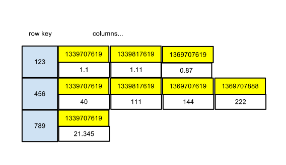
Metric schedule ids are used as the row keys. The column names are the timestamp for each data point. And the column value is the value of the data point. This is a very common design for time series data with Cassandra. Querying for a time slice or the most recent value are easy, fast and efficient operations.
Composites provide for nesting of components in the column name or in the row key. The nesting can be arbitrarily deep. The grouping made available with composites make indexes more efficient. In terms of implementation, there is a composite comparator which is a comparator composed of other comparators. The following CLI script makes use of composites:
create column family one_hour_metric_data
    with comparator = 'CompositeType(DateType, Int32Type)' and
    default_validation_class = DoubleType and
    key_validation_class = Int32Type;
The one_hour_metric_data column family is dynamic since it does not define any columns up front. It uses a composite for the column names. The column name is a composite that consists of a timestamp and an integer code indicating the aggregate type, e.g., max, min, or avg. And here is some sample data from one_hour_metric_data being retrieved using the Cassandra CLI,
[default@rhq] get one_hour_metric_data[10261];
=> (column=2012-06-14 16:00:00-0400:0, value=8528.610195208777, timestamp=1339707619159001, ttl=1209600)
=> (column=2012-06-14 16:00:00-0400:1, value=7914.6, timestamp=1339707619159002, ttl=1209600)
=> (column=2012-06-14 16:00:00-0400:2, value=8221.605097604388, timestamp=1339707619159000, ttl=1209600)
The first entry in the tuple, column, is the column name. It may be a bit difficult to see because of the date formatting, but a colon separates the timestamp and integer values that make up the column name. Next is the column value followed by client supplied timestamp and TTL.
Indexes
As with other databases, indexes are integral to making queries efficient. I want to call out indexing separately though since techniques in Cassandra differ significantly from those in either MongoDB or in PostgreSQL. Cassandra does offer limited support for secondary indexes; however, custom-built indexes are still the norm. Let's consider a users column family with some rows that look like,
users = {
  "jsanda" : {
    "fname": "John",
    "lname": "Sanda",
    "email": "jsanda@redhat.com",
    "address": "Main St.",
    "state": "NC",
    "department": "Engineering",
    ...
  },

  "jdoe": {
    "fname": "John",
    "lname": "Doe",
    "email": "john.doe@redhat.com",
    "address": "Smith St.",
    "state": "TX",
    "department": "Finance",
    ...
  }
}
JSON-style notation is commonly used technique for illustrating and describing column families. In this example, we have the users column family with the username as keys. For a column family such as this, columns are likely to be defined statically; however, that need not be the case. Querying for a user is easy provided you have the username. Suppose you want to search for users by last name. To do this efficiently we create an index.
One strategy is to utilize wide rows:
indexes = {
  "users_by_lname" : {
    "Sanda": "jsanda",
    "Doe": "jdoe",
    ...
  }
}
Here we have an indexes column family where each row represents a different index. Given a last name, we can quickly and efficiently look up the username. This row could easily wind up with thousands or millions of columns depending on the number of users we are storing. Now suppose we want search for users by state. We can utilize another technique whereby a single index is stored in a column family:
users_by_state = {
  "NC": {
    "jsanda": null,
    "jones": null,
    ....
  }

  "TX": {
    "jdoe": null,
    ...
  }
}
With this technique, usernames are partitioned by state. The index data will be distributed across the cluster whereas with a wide row, the data is not partitioned since it is all stored under a single key. Let's revisit the users_by_lname index. What if we have multiple users with the same last name? We can utilize composites to ensure we have unique values for our column names:
indexes = {
  "users_by_lname" : {
    {"Sanda", "jsanda@redhat.com"}: "jsanda",
    {"Doe", "john.doe@redhat.com"}: "jdoe",
    {"Smith", "jane.smith@redhat.com"}: "jsmith",
    {"Smith", "doug.smith@redhat.com"}: "dsmith"
    ...
  }
}
Fault Tolerance
Cassandra has no single point of failure. Any node can service a read or write request. Like other Dynamo systems, it is designed to be highly available and resilient to failure.
The only time Cassandra will fail a write entirely is when too few replicas are alive when the coordinator receives the request. See this article for more details.
Gossip
Cassandra uses a gossip protocol to learn about the nodes in the cluster as well as state information. Gossip runs every second. A node uses gossip state to locally perform failure detection. The node will determine if other nodes in the cluster are up or down. Failure detection is also used to avoid routing requests to unreachable nodes.
Hinted Handoff
If a node is down or fails to acknowledge a write, the coordinating node will store a hint. The hint consists of the destination node along with the missed operation. Hints are replayed as soon as possible once the down node becomes available. Hinted handoffs are disabled by default. Hints are stored for at most an hour by default. If the node does not become available within that time, Cassandra assumes the node is permanently down. If the node does come back up after that extended period, it is best to run repair on it.
Read Repair
Consistency
Cassandra offers tunable consistency. Different consistency levels can be specified for individual read and write operations. A write with a consistency level of QUORUM means that the write succeed on a quorum of the replica nodes in order for the write to be considered successful A write with a consistency level of ONE in contrast, only needs to be successful on a single node in order for the write to be considered successful.
With reads, the consistency level determines the number of nodes that must respond in order for the read to be successful. A read with a consistency level of QUORUM will return when a quorum of replicas has responded to the request. A read with a consistency level of ONE will return when a single node responds to the request.
Replication
Replication is configured at the schema (i.e., key space) level in Cassandra. This is specified as an option (replication_factor) when creating the key space. If you start out with a one or two node cluster and later expand, it is likely that you may want to increase the replicate_factor at some point. If the replication_factor is increased on a live cluster, then you need to run read repair on each node to ensure that each one has the correct data. Until repair finishes on all of the nodes, you can:
-
read at consistency level QUORUM or ALL to make sure that a replica that actually has the data takes part in the request
-
read at a lower consistency level, accepting that some requests will fail
-
take down time while the repair runs
Data Processing
There is nothing in Cassandra today for doing any kind of data processing server side. For instance, if you have a row of integer values that you want to sum, you will have to perform that client-side. It is possible that support for running application code on the server may be added in the future. There is CASSANDRA-1311 which discusses adding support for triggers. Many Cassandra users will rely on Hadoop for data processing needs like analytics. Cassandra provides rich Hadoop integration, more so than a lot of other databases. Here is a brief summary of the Hadoop integration that is available:
-
Cassandra can be used as a MapReduce input source. Jobs can read data from Cassandra.
-
Cassandra can be used as a MapReduce output source. Jobs can write data to Cassandra.
-
Cassandra implements HDFS to achieve input data locality.
-
Pig queries can be run against Cassandra.
DataStax has taken the Hadoop integration even further with its enterprise edition. They have a full Hadoop distribution that runs embedded inside of Cassandra. Instead of running multiple processes for the different nodes that comprise a Hadoop cluster, those nodes run in separate threads inside a Cassandra node. DataStax Enterprise however is free only for development use.
The primary need in RHQ for data processing with respect to metrics and other time series data is compression. This involves calculating simple aggregates (max, min, avg.) for numeric metrics in each of the buckets (i.e., raw, 1hr, 6hr, 24hr) that we maintain. The compression is done every hour in a background job. With the existing RDBMS implementation, computing the aggregates is done server-side by the database. For a Cassandra-based implementation we would do it client-side in the RHQ server. Utilizing the concurrency features provided by the application server and JVM, we should be able to achieve a high level of throughput capable of handling heavy loads. If/when we reach a point where doing the work on the RHQ server (or servers) does not scale, then we should consider Hadoop integration, but only as a future enhancement if in fact needed. I will provide more specific thoughts and details around the data processing in a Cassandra design document (yet to be created).
MongoDB
MongoDB is an open source document-oriented database that is written in C++.
Performance
MongoDB offers high performance for both reads and writes. MongoDB is similar to relational databases in that it uses B-tree indexes. A good indexing strategy can make queries extremely fast. MongoDB uses memory-mapped files for all disk IO. It relies on the operating system to handle caching and to determine what pages pages should be in memory and what pages can be swapped out to disk. For writes, MongoDB updates the journal where operations are recorded, and then it updates the pages for the effected collections and indexes. The journal is periodically flushed to disk. I believe it is flushed every 100 ms by default.
MongoDB relies on the operating system to handle caching and to determine which pages should be resident in memory. When the work set fits into memory both reads and write will be fast. Performance will suffer when there are page faults that require that operating system to swap pages in from disk to fulfill read or write requests. Other than scaling up by increasing memory, another solution to address inadequate memory is to increase overall capacity by scaling out horizontally.
Scalability
MongoDB's solution for horizontal scaling is sharding. Sharding partitions data evenly across machines at the collection level. To shard a collection you have to specify a shard key. For metric data, the schedule id would be a logical choice or starting point. Let's consider a simple example to see how this works. Suppose we have three shard servers - S1, S2, and S3. And suppose we are storing metrics for schedule ids 1 through 90. Metric data for schedules 1 through 30 would be stored on S1, data for schedules 31 through 60 would be stored on S2, and data for schedules 61 through 90 would be stored on S3.
Sharded data is stored in chunks. A chunk simply point is a continuous range of data from a collection. The metric data on server S1 for example would constitute a chunk. When the load on a shard servers gets too large it is necessary to rebalance the load across the cluster. By default chunks have a maximum size of 64 MB. Once a chunk has reached the maximum size, it is split into two new chunks. The balancer is a background task whose job is to keep the number of chunks evenly distributed across the cluster. Rebalancing will also occur when shards are added to or removed from the cluster. Splitting and migrating chunks happens automatically in the background, completely transparent to clients.
There are several different components involved involved in a sharded cluster. The following diagram the components and there interactions: 
Here is a brief description of each of the components involved.
Shards
Each shard consists of one or more servers, i.e., mongod processes. For production, it is recommended to use a replica set for each shard. This is why in the diagram you see three mongod processes per shard. Note that one of those mongod processes could be an arbiter instead of a full replica.
Config DBs
The config servers store contains meta data for each shard server as well as information about chunks. Each config server maintains a full copy of the chunk data and a two-phase commit protocol is used to ensure that the data is consistent across server. If any of the config servers go down, the config meta data becomes read only; however, you can still write to and read from the shards. If a config server goes down and the meta data becomes read only, that would seem to imply that certain operations cannot take place including,
-
rebalancing chunks across the cluster
-
adding/removing shards
I am not 100% certain as to whether or not those operations cannot be performed while a config server is down.
TODO
Find out what if any cluster operations cannot be performed while a config server is down.
The last thing to mention about config servers that it is recommended to run three of them for production use. The replication protocol used for config servers is optimized for three machines.
Routing Processes (mongos)
The mongos process is basically a lightweight proxy. It routes requests to the appropriate servers and takes care of merging results back to clients. They maintain no persistent state of their own and have a small enough footprint that they do not require their own dedicated hardware. Multiple mongos processes can be run as there is no coordination between them. Any mongos process can service any client request.
Administration and Management
MongoDB ships with several external utilities to assist with administrative tasks. Many of those are just wrappers around built-in commands that are available both from the mongo shell as well as from the different language drivers. There are monitoring commands like collStats and serverStatus. The former provides detailed information about a collection such as the number of documents, the average document size, and sizes of indexes. The latter command, serverStatus, provide detailed monitoring information for the server as a whole for things like locks, memory usage, and indexes.
Administrative Tasks
In this section I want to call attention to administrative tasks of which I am aware. Some tasks might only be applicable in certain deployment scenarios. For example, if you using sharding, there might be tasks specific to the config servers. Unless noted otherwise, the following tasks apply to a server in any deployment scenarios.
Backups
There are two ways of performing backups. The first is using the mongodump utility. This export the database contents into BSON files. Indexes are not included in the dump. This means indexes will have to be rebuilt when you restore. The other, more popular approach is file-based backups where you simply create copies of data files. The advantages of file-based backups is that often faster than mongodump and indexes are included. The big disadvantage is that it requires locking the entire database. The copied files could become corrupted if the database is not locked. Typically the backup operation will be performed on a secondary node so that the primary remains available while the backup is running.
Compaction
The data files on disk will grow over time. MongoDB does not manage space as efficiently as a RDBMS in order to achieve better write performance. You will want to periodically run compaction. Compaction rewrites data files and rebuilds indexes. It can be done on a per-collection basis. The compact command has been designed to run on a live secondary. Once compaction has been run on all secondaries, it can be run against the primary while one of the already compacted secondaries takes over as primary. Note that running compaction on the primary requires locking the database.
Clustering Architecture
MongoDB uses a master/slave architecture where all writes must go to the master nodes. Reads can go either to the master or to slave nodes. More details on clustering are provided in the sections on scalability and replication.
Data Model
MongoDB is a schemaless database. Unlike relational databases where a schema is defined up front and is fixed, MongoDB is completely dynamic. Collections in MongoDB are analogous to tables in relational database. A collection consists of documents. The documents are represented and stored in BSON which is a binary-encoded form of JSON. Just as with JSON, documents can have a rich structure. Documents and arrays can be nested arbitrarily deep. MongoDB does not require documents in a collection to have the same fields or even fields of the same name between documents to be of the same type; however, in practice the structure of documents in a collection is usually fairly consistent. This rich document structure maps much better to object oriented models than do relational data models.
Here is what a document for raw metric data might look like:
{
  _id: ObjectId("4e77bb3b8a3e000000004f7a"),
  scheduleId: 123,
  timestamp: 1339707619159001,
  value: 1.414421356237
}
This is pretty self-explanatory. Here is a more complex example that illustrates a drift change set.
{ "_id": ObjectId("4f5c171303649e4c22b96671"),
  "className": "org.rhq.enterprise.server.plugins.drift.mongodb.entities.MongoDBChangeSet",
  "ctime": NumberLong("1331435283586"),
  "version": 1,
  "category": "DRIFT",
  "driftDefId": 10021,
  "driftHandlingMode": "normal",
  "resourceId": 10001,
  "driftDefName": "DRIFT-1-PINNED",
  "files": [
    {
      "idx": 0,
      "ctime": NumberLong("1331435283586"),
      "category": "FILE_ADDED",
      "path": "test_script",
      "directory": "./",
      "newFileHash": "d00447de74e70c236d2870d8b4d06376c3454a2d5602fbd622dc6f763706943d"
    },
    {
      "idx": 1,
      "ctime": NumberLong("1331435283598"),
      "category": "FILE_ADDED",
      "path": "underscore-min.js",
      "directory": "./",
      "newFileHash": "42d8fad13bc28fc726775196ec9ab953febf9bde175c5845128361c953fa17f4"
    }
  ]
}
The interesting thing to note about the change set document is the files array. It is an array of nested documents or objects. Each of those nested objects represents an instance of drift. In the relational model, drift instances are stored in their own table, and we have a 1-to-many relationship between the change set and drift tables. In the MongoDB model, we store the change set and drift as a single document. For a change set with 4 drift instances, you have to do 5 inserts in the relational model. With the MongoDB model, you only have to do one insert. MongoDBs rich query language provides the flexibility to exclude the files array from query results when it is not needed. You can also retrieve a subset of the array.
Fault Tolerance
MongoDB provides fault tolerance through replica sets. See the section on replication below for more details.
Consistency
MongoDB provides strong consistency by allowing only the primary to receive writes. If strong consistency is not important, then you can send read requests to secondaries. The replication from primary to secondary is asynchronous, which means you have read uncommitted type semantics. For example, you can send a write request to the primary to insert a document, immediately query for that document from a secondary, and then have an empty result set returned. MongoDB provides the ability to verify that a write propagates to secondaries as explained here. You can for example specify that a write block (on the client side) until the data has reach a majority of the nodes. At the driver level, this is controlled by setting the WriteConcern on write requests.
Replication
MongoDB's solution for replication is replica sets. Replica sets provide full, asynchronous replication and with automatic failover. A replica set consists of two or more nodes that are full copies of one another. One of the nodes is automatically elected primary or master; however I believe it is possible to manually specify which node should be primary. Because of this election process to determine the primary, in practice you will have a minimum of three nodes in a replica set, and it is good practice to have an odd number to avoid ties in the election process. One of the nodes can be an arbiter where its only role is to be a tie breaker in the election process. An arbiter node is unique in that it does not maintain a copy of the data like the other nodes do.
It is important to understand that only the primary services write requests. This means that if a replica set has an even number of nodes and if the election process results in a tie, then writes will fail until a primary is elected. If this happens, then you would need to execute an administrative command to manually appoint a node as primary.
When the primary fails, the election will take place making a secondary the new primary. If/when the former primary comes back up and rejoins the replica set, it will rejoin as a secondary. As for client code, the driver will detect when the primary has change and redirect writes accordingly, thus eliminating the need for changes to client code.
Data Processing
MongoDB provides a couple options for server-side data processing. It has MapReduce. The map and reduce functions are defined in JavaScript. There have been a lot of reports of poor performance as the map and reduce functions are executed entirely through the JavaScript interpreter. Another caveat of this is that the execution model is single threaded. In version 2.1 MongoDB introduced the Aggregation Framework which woud likely be a better option. It is more performant than MapReduce, does not require writing custom JavaScript functions, and allows pipelines to be defined through standard driver APIs.
Summary
Due to the challenges we faced with the Infinispan data model we decided it was not a good fit for our needs. In terms of management, performance, and scalability, it is an excellent fit. It is not a good fit though meeting our functional requirements. In the remainder of this section, I will focus on Cassandra and MongoDB, particularly around the areas of management, performance, and developer tools.
Management
MongoDB provides a rich set of built-in functions and collections that allow you to effectively manage and monitor your databases and mongod servers. Those functions are accessible through driver APIs. I think we can manage a single server or even a replica set pretty effectively. For example, consider doing backups and running compactions. We can do a good job of automating those tasks while minimizing down time (assuming you are running a replica set). My bigger concerns are around sharding. As was pointed out, we are talking about 10 or 11 processes at a minimum. That is a lot of moving parts. That large number of moving parts is the sole reason I have avoided Hadoop as an option.
Cassandra's clustering architecture is much simpler in so far as it is a single process per node. That is a big win. Let's consider some of the administrative tasks. Minor compaction runs automatically in the background. It is configurable and can be tuned. With MongoDB, you have to promote a secondary while perform maintenance if you want to avoid downtime. This is less of an issue with Cassandra since any node can handle read or write requests.
I will go through some uses cases we would have to support in order to black box this new database.
First, let's consider doing backups or compaction. Because of the database locking involved, MongoDB recommends running those tasks against a secondary node, and then when the task has completed, promote the node to primary. Whether it is Cassandra or MongoDB, we need to support a single node install. For a single node MongoDB deployment, we are looking downtime in order to do routine maintenance. That's bad because we want the metrics database to be highly available.
Secondly, let's talk more about replica sets. Assume we running with a replica set. Now we can perform the maintenance tasks while avoiding downtime. Remember that only the primary handles writes. It's not a question of if but a question of when a primary goes down and a secondary is not promoted, how quickly can we intervene to manually promote a secondary. By manually, I mean the RHQ server and/or agent as opposed to the end user. I am not sure how likely this scenario is, but it is certainly something we would have to account for. Cassandra is a P2P system where any node can receive reads or writes. Every node is the same in that regard, and this reduces and simplifies the use cases we have to handle.
As a third example, let's consider increasing capacity to scale writes. Assume we are already running a replica set. To scale writes though, we need to go to sharding. This means we want to automate the process of deploying and setting another replica set (maybe more), preferably three config servers, and one or more mongos routers. Again Cassandra's simpler P2P architecture makes this easier. When we need to increase capacity with Cassandra, we just add more nodes as needed.
We will stick with sharding for a final example. The config servers maintain meta data for the shards. The meta includes things like the locations and sizes of chunks (i.e., range of data). They all provide the information necessary for mongos to know where to route reads and writes. If a config server goes down, that meta data becomes read only. Chunk splitting and migration will be inoperable. If all config servers go down, the entire cluster could become inoperable. This is another scenario that we do not have to worry about with Cassandra.
All in all, I think Cassandra wins out for management. The simpler clustering architecture is a big plus, and the fact that it runs on the JVM gives us a big advantage as well since we already have a lot of infrastructure, tooling, and experience in monitoring the JVM.
Performance
First off, let me say that I am confident that we can achieve higher than acceptable levels of performance with either Cassandra or with MongoDB. Achieving high read performance with MongoDB might be easier (at least early on) since it uses the same B-tree indexes used in relational databases. MongoDB' solid support for secondary indexes could very well ease performance management. While there is growing support for secondary indexes in Cassandra, it is likely that we will still rely heavily on custom-built indexes. Suppose we have to provide a customer patch with some new indexes to address performance problems. With MongoDB, that wouldn't require anything more than a simple script whereas with Cassandra, we are likely looking at application code changes. Because of this, I give the edge to MongoDB for read performance even though high performances reads are possible with Cassandra.
For write performance, Cassandra is a clear winner. Writes are a constant time operation in Cassandra. With MongoDB, if your working set, and your indexes in particular, do not fit into memory, performance is likely to degrade quickly. Another aspect of Cassandra that allows you to achieve high write throughput is its use lock-free algorithms and data structures. MongoDB on the other hand does rely on locks.
In terms of space performance (disk, memory), I give Cassandra the edge. MongoDB relies completely on memory-mapped IO and will use all available memory. It does not actually actively use all memory; however, this does make me concerned that high memory usage could be problematic. Cassandra relies primarily on the JVM heap for memory. It does rely on the OS virtual memory manger for caching like MongoDB does, but Cassandra uses a specified amount of space as opposed to all available memory. In terms of disk usage, Cassandra stores data files on disk in a compressed format. in addition to reducing the foot print on disk, this actually also improves read performance. MongoDB does not currently compress data on disk. MongoDB pre-allocates data files to improve performance. When a new file is needed, its size will be double that of the previous data file. The sizes are doubled up to 2 GB. Both Cassandra and MongoDB trade disk space for performance. Because MongoDB does not compress data files and because of its aggressive approach for pre-allocating data files, I think Cassandra wins in terms of disk usage.
For metrics, call time, and events, we are talking about a lot more writes than reads and storing a lot of data. Overall, Cassandra wins out for performance here as this data is very write-heavy.
Developer/Support Tooling
I want to call out support separately from management. In the management section I am referring to day to day maintenance operations that we need to effectively automate so that we can black box the database. With support, I am referring to those user/customer issues that go beyond the management tools we provide in the product. In those situations, we often rely on the same tools that we use for development.
MongoDB is very, very developer friendly. If you are coming from a clean slate, not having worked with either MongDB or with Cassandra, I have little to no doubt that you can become more productive with MongoDB more quickly than you will with Cassandra. MongoDB has a larger community and really solid documentation. Though I should point out that in my experience I have found the community support for both to be really good. It is easy to transition to the document data model. In fact, the flexible data model maps much more cleanly to OO data models than do relational models. The Java driver is stable and well-documented. I have used the type-mapping library Morphia that is layered on top of the driver. It is very easy and intuitive to use.
Cassandra's data model by comparison is less intuitive and brings with it a steeper learning curve. It provides a Thrift based API for client use, which is actually discouraged because of it not being developer-friendly. Developers are instead encouraged to use higher-level libraries that layer on top of the Thrift API. I have used Hector. It is stable and well documented. The core Cassandra team is pushing CQL really hard as the primary client interface. It lacks some critical features that would be necessary for full adoption right now, but it has the potential to go a long way in making Cassandra more developer friendly.
Another key aspect to consider for development and for support is that Cassandra is implemented in Java whereas MongoDB is implemented in C++. This gives Cassandra a big advantage that cannot be understated. We can load the source in our IDEs along side RHQ code, step through a running Cassandra server in the debugger, or utilize tools like MAT (http://www.eclipse.org/mat/) to analyze heap dumps. This can be invaluable for providing support.
Conclusion
Cassandra and MongoDB are impressive technologies with a lot to offer. I believe that Cassandra is a better fit for our needs and propose we move in that direction.