Chapter 9. Federated Planning

Teiid at its core is a federated relational query engine. This query engine allows you to treat all of your data sources as one virtual database and access them in a single SQL query. This allows you to focus on building your application, not on hand-coding joins, and other relational operations, between data sources.

9.1. Overview

When the query engine receives an incoming SQL query it performs the following operations:

Parsing - validate syntax and convert to internal form
Resolving - link all identifiers to metadata and functions to the function library
Validating - validate SQL semantics based on metadata references and type signatures
Rewriting - rewrite SQL to simplify expressions and criteria
Logical plan optimization - the rewritten canonical SQL is converted into a logical plan for in-depth optimization. The Teiid optimizer is predominantly rule-based. Based upon the query structure and hints a certain rule set will be applied. These rules may trigger in turn trigger the execution of more rules. Within several rules, Teiid also takes advantage of costing information. The logical plan optimization steps can be seen by using the OPTION DEBUG clause and are described in the query planner section.
Processing plan conversion - the logic plan is converted into an executable form where the nodes are representative of basic processing operations. The final processing plan is displayed as the query plan .

The logical query plan is a tree of operations used to transform data in source tables to the expected result set. In the tree, data flows from the bottom (tables) to the top (output). The primary logical operations are select (select or filter rows based on a criteria), project (project or compute column values), join , source (retrieve data from a table), sort (ORDER BY), duplicate removal (SELECT DISTINCT), group (GROUP BY), and union (UNION).

For example, consider the following query that retrieves all engineering employees born since 1970.

Example 9.1. Example query

SELECT e.title, e.lastname FROM Employees AS e JOIN 
Departments AS d ON e.dept_id = d.dept_id WHERE year(e.birthday) >= 1970 AND d.dept_name = 'Engineering'

Logically, the data from the Employees and Departments tables are retrieved, then joined, then filtered as specified, and finally the output columns are projected. The canonical query plan thus looks like this:

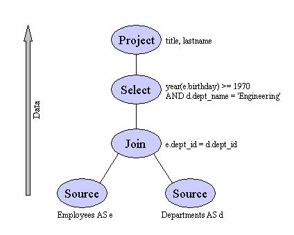
Data flows from the tables at the bottom upwards through the join, through the select, and finally through the project to produce the final results. The data passed between each node is logically a result set with columns and rows.

Of course, this is what happens logically , not how the plan is actually executed. Starting from this initial plan, the query planner performs transformations on the query plan tree to produce an equivalent plan that retrieves the same results faster. Both a federated query planner and a relational database planner deal with the same concepts and many of the same plan transformations. In this example, the criteria on the Departments and Employees tables will be pushed down the tree to filter the results as early as possible.

In both cases, the goal is to retrieve the query results in the fastest possible time. However, the relational database planner does this primarily by optimizing the access paths in pulling data from storage.

In contrast, a federated query planner is less concerned about storage access because it is typically pushing that burden to the data source. The most important consideration for a federated query planner is minimizing data transfer.

9.2. Federated Optimizations

9.2.1. Access Patterns

Access patterns are used on both physical and virtual sources to specify the need for criteria against a set of elements. Failure to supply the criteria will result in a planning error, rather than a run-away source query. Access patterns can be applied in a set such that only one of the access patterns is required to be satisfied.

Currently any form of criteria may satisfy an access pattern as long as it contains references to affect elements.

9.2.2. Pushdown

In federated database systems pushdown refers to decomposing the user level query into source queries that perform as much work as possible on their respective source system. Pushdown analysis requires knowledge of source system capabilities, which is provided to Teiid though the Connector API. Any work not performed at the source is then processed in Federate's relational engine.

Based upon capabilities, Teiid will manipulate the query plan to ensure that each source performs as much joining, filtering, grouping, etc. as possible. In may cases, such as with join ordering, planning is a combination of standard relational techniques and, cost based and heuristics for pushdown optimization.

Criteria and join push down are typically the most important aspects of the query to push down when performance is a concern. See Query Plans on how to read a plan to ensure that source queries are as efficient as possible.

9.2.3. Dependent Joins

A special optimization called a dependent join is used to reduce the rows returned from one of the two relations involved in a multi-source join. In a dependent join, queries are issued to each source sequentially rather than in parallel, with the results obtained from the first source used to restrict the records returned from the second. Dependent joins can perform some joins much faster by drastically reducing the amount of data retrieved from the second source and the number of join comparisons that must be performed.

The conditions when a dependent join is used are determined by the query planner based on access patterns, hints, and costing information.

Teiid supports the MAKEDEP and MAKENOTDEP hints. Theses are can be placed in either the OPTION clause or directly in the FROM clause . As long as all can be met, the MAKEDEP and MAKENOTDEP hints override any use of costing information.

Tip

The MAKEDEP hint should only be used if the proper query plan is not chosen by default. You should ensure that your costing information is representative of the actual source cardinality. An inappropriate MAKEDEP hint can force an inefficient join structure and may result in many source queries.

9.2.4. Copy Criteria

Copy criteria is an optimization that creates additional predicates based upon combining join and where clause criteria. For example, equi-join predicates (source1.table.column = source2.table.column) are used to create new predicates by substituting source1.table.column for source2.table.column and vice versa. In a cross source scenario, this allows for where criteria applied to a single side of the join to be applied to both source queries

The optional join hint indicates to the optimizer that a join clause should be omitted if none of its columns are used in either user criteria or output columns in the result. This hint is typically only used in view layers containing multi-source joins.

The optional join hint is applied as a comment on a join clause.

Example 9.2. Example Optional Join Hint

select a.column1, b.column2 from a inner join /* optional */ b on a.key = b.key

Suppose that the preceding example defined a view layer X. If X is queried in such a way as to not need b.column2, then the optional join hint will cause b to be omitted from the query plan. The result would be the same as if X were defined as:

select a.column1 from a

Tip

When a join clause is omitted, the relevant join criteria is not applied. Thus it is possible that the query results may not have the same cardinality or even the same row values as when the join is fully applied.

9.2.8. Standard Relational Techniques

Teiid also incorporates many standard relational techniques to ensure efficient query plans.

Rewrite analysis for function simplification and evaluation.
Boolean optimizations for basic criteria simplification.
Removal of unnecessary view layers.
Removal of unnecessary sort operations.
Advanced search techniques through the left-linear space of join trees.
Parallelizing of source access during execution.

9.3. Federated Failure Modes

9.3.1. Partial Results

Teiid provides the capability to obtain "partial results" in the event of data source unavailability. This is especially useful when unioning information from multiple sources, or when doing a left outer join, where you are 'appending' columns to a master record but still want the record if the extra info is not available.

If one or more data sources are unavailable to return results, then the result set obtained from the remaining available sources will be returned. In the case of joins, an unavailable data source essentially contributes zero tuples to the result set.

9.3.1.1. Setting Partial Results Mode

Partial results mode is off by default but can be turned on by default for all queries in a Connection with either setPartialResultsMode("true") on a DataSource or partialResultsMode=true on a JDBC URL. In either case, partial results mode may be overridden on a per-query basis by setting the execution property on the Statement. To set this property, cast to the Teiid Statement JDBC API extension interface com.metamatrix.jdbc.api.Statement

Example 9.3. Example - Setting Partial Results Mode

Statement statement = ...obtain statement from Connection... 

com.metamatrix.jdbc.api.Statement mmStatement = 
  (com.metamatrix.jdbc.api.Statement) statement;
  
mmStatement.setExecutionProperty( 
  ExecutionProperties.PROP_PARTIAL_RESULTS_MODE, "true");

This property can be set before each execution (via an execute method) on a Statement (or PreparedStatement or CallableStatement).

9.3.1.2. Source Unavailability

A source is considered to be 'unavailable' if the connector binding associated with the source issues an exception in response to a query. The exception will be propagated to the query processor, where it will become a warning in the result set.

Warning

Since Teiid supports multi-source cursoring, it is possible that the unavailability of a data source will not be determined until after the first batch of results have been returned to the client. This can happen in the case of unions, but not joins. In this situation, there will be no warnings in the result set when the client is processing the first batch of results. The client will be responsible for periodically checking the status of warnings in the results object as results are being processed, to see if a new warning has been added due to the detection of an unavailable source. [Note that client applications have no notion of ‘batches’, which are purely a server-side entity. Client apps deal only with records.]

For each source that is excluded from a query, a warning will be generated describing the source and the failure. These warnings can be obtained from the Statement.getWarnings() method. This method returns a SQLWarning object but in the case of "partial results" warnings, this will be an object of type com.metamatrix.jdbc.api.PartialResultsWarning. This class can be used to obtain a list of all the failed connectors by name and to obtain the specific exception thrown by each connector.

Example 9.4. Example - Printing List of Failed Sources

statement.setExecutionProperty( PROP_PARTIAL_RESULTS_MODE, "true"); 
ResultSet results = statement.executeQuery("SELECT Name FROM Accounts"); 
SQLWarning warning = statement.getWarnings(); 
if(warning instanceof PartialResultsWarning) { 
  PartialResultsWarning partialWarning = (PartialResultsWarning)warning; 
  Collection failedConnectors = partialWarning.getFailedConnectors(); 
  Iterator iter = failedConnectors.iterator(); 
  while(iter.hasNext()) { 
    String connectorName = (String) iter.next(); 
    SQLException connectorException = partialWarning.getConnectorException(connectorName); 
    System.out.println(connectorName + ": " + ConnectorException.getMessage();
  }
}

9.4. Query Plans

When integrating information using a federated query planner, it is useful to be able to view the query plans that are created, to better understand how information is being accessed and processed, and to troubleshoot problems.

A query plan is a set of instructions created by a query engine for executing a command submitted by a user or application. The purpose of the query plan is to execute the user's query in as efficient a way as possible.

9.4.1. Getting a Query Plan

You can get a query plan any time you execute a command. The SQL options available are as follows:

OPTION SHOWPLAN - Returns the plan in addition to any results
OPTION PLANONLY - Returns the plan, does not execute the command though

With the above options, the query plan is available from the Statement object by casting to the com.metamatrix.jdbc.api.Statement interface.

Example 9.5. Retrieving a Query Plan

ResultSet rs = statement.executeQuery("select ...");
com.metamatrix.jdbc.api.Statement mmstatement = (com.metamatrix.jdbc.api.Statement)statement;
PlanNode queryPlan = mmstatement.getPlanDescription();
System.out.println(XMLOutputVisitor.convertToXML(queryPlan);

The query plan is made available automatically in several of Teiid's tools.

Statistic	Description	Units
Node Output Rows	Number of records output from the node	count
Node Process Time	Time processing in this node only	millisec
Node Cumulative Process Time	Elapsed time from beginning of processing to end	millisec
Node Cumulative Next Batch Process Time	Time processing in this node + child nodes	millisec
Node Next Batch Calls	Number of times a node was called for processing	count
Node Blocks	Number of times a blocked exception was thrown by this node or a child	count

In addition to node statistics, some nodes display cost estimates computed at the node.

Cost Estimates	Description	Units
Estimated Node Cardinality	Estimated number of records that will be output from the node; -1 if unknown	count

9.5. Query Planner

For each sub-command in the user command an appropriate kind of sub-planner is used (relational, XML, XQuery, procedure, etc).

Each planner has three primary phases:

Generate canonical plan
Optimization
Plan to process converter - converts plan data structure into a processing form

9.5.1. Relational Planner

The GenerateCanonical class generates the initial (or “canonical” plan). This plan is based on the typical logical order that a SQL query gets executed. A SQL select query has the following possible clauses (all but SELECT are optional): SELECT, FROM, WHERE, GROUP BY, HAVING, ORDER BY, LIMIT. These clauses are logically executed in the following order:

FROM (read and join all data from tables)
WHERE (filter rows)
GROUP BY (group rows into collapsed rows)
HAVING (filter grouped rows)
SELECT (evaluate expressions and return only requested columns)
INTO
ORDER BY (sort rows)
LIMIT (limit result set to a certain range of results)

These clause translate into the following types of planning nodes:

FROM: Source node for each from clause item, Join node (if >1 table)
WHERE: Select node
GROUP BY: Group node
GROUP BY: Group node
SELECT: Project node and DupRemoval node (for SELECT DISTINCT)
INTO: Project node with a SOURCE Node
INTO: Project node with a SOURCE Node
LIMIT: Limit node
UNION, EXCEPT, INTERSECT: SetOp Node

There is also a Null Node that can be created as the result of rewrite or planning optimizations. It represents a node that produces no rows

Relational optimization is based upon rule execution that evolves the initial plan into the execution plan. There are a set of pre-defined rules that are dynamically assembled into a rule stack for every query. The rule stack is assembled based on the contents of the user’s query and its transformations. For example, if there are no virtual layers, then RuleMergeVirtual, which merges virtual layers together, is not needed and will not be added to the stack. This allows the rule stack to reflect the complexity of the query.

Logically the plan node data structure represents a tree of nodes where the source data comes up from the leaf nodes (typically Access nodes in the final plan), flows up through the tree and produces the user’s results out the top. The nodes in the plan structure can have bidirectional links, dynamic properties, and allow any number of child nodes. Processing plan nodes in contrast typical have fixed properties, and only allow for binary operations - due to algorithmic limitations.

Below are some of the rules included in the planner:

RuleRemoveSorts - removes sort nodes that do not have an effect on the result. This most common when a view has an non-limited ORDER BY.
RulePlaceAccess - insert an Access node above every physical Source node. The source node represents a table typically. An access node represents the point at which everything below the access node gets pushed to the source. Later rules focus on either pushing stuff under the access or pulling the access node up the tree to move more work down to the data sources. This rule is also responsible for placing .
RulePushSelectCriteria - pushes select criteria down through unions, joins, and views into the source below the access node. In most cases movement down the tree is good as this will filter rows earlier in the plan. We currently do not undo the decisions made by PushSelectCriteria. However in situations where criteria cannot be evaluated by the source, this can lead to sub optimal plans.
One of the most important optimization related to pushing criteria, is how the criteria will be pushed trough join. Consider the following plan tree that represents a subtree of the plan for the query "select ... from A inner join b on (A.x = B.x) where A.y = 3"
```
          SELECT (B.y = 3)
           |
          JOIN - Inner Join on (A.x = B.x
         /     \    
      SRC (A)   SRC (B)
```
Note: SELECT nodes represent criteria, and SRC stands for SOURCE.
It is always valid for inner join and cross joins to push (single source) criteria that are above the join, below the join. This allows for criteria originating in the user query to eventually be present in source queries below the joins. This result can be represented visually as:
```
          JOIN - Inner Join on (A.x = B.x)
          /    \
         /   SELECT (B.y = 3)
        |        |
      SRC (A)   SRC (B)
```
The same optimization is valid for criteria specified against the outer side of an outer join. For example:
```
          SELECT (B.y = 3) 
           |
          JOIN - Right Outer Join on (A.x = B.x)
         /     \    
      SRC (A)   SRC (B)
```
Becomes
```
          JOIN - Right Outer Join on (A.x = B.x)
          /    \
         /   SELECT (B.y = 3)
        |        |
      SRC (A)   SRC (B)
```
However criteria specified against the inner side of an outer join needs special consideration. The above scenario with a left or full outer join is not the same. For example:
```
          SELECT (B.y = 3)
           |
          JOIN - Left Outer Join on (A.x = B.x)
         /     \    
      SRC (A)   SRC (B)
```
Can become (available only after 5.0.2):
```
          JOIN - Inner Join on (A.x = B.x)
          /    \
         /   SELECT (B.y = 3)
        |        |
      SRC (A)   SRC (B)
```
Since the criterion is not dependent upon the null values that may be populated from the inner side of the join, the criterion is eligible to be pushed below the join – but only if the join type is also changed to an inner join.
On the other hand, criteria that are dependent upon the presence of null values CANNOT be moved. For example:
```
          SELECT (B.y is null)
           |
          JOIN - Left Outer Join on (A.x = B.x)
         /     \   
      SRC (A)   SRC (B)
```
This plan tree must have the criteria remain above the join, since the outer join may be introducing null values itself. This will be true regardless of which version of Teiid is used.
RulePushNonJoinCriteria – this rule will push criteria out of an on clause if it is not necessary for the correctness of the join.
RuleRaiseNull – this rule will raise null nodes to their highest possible point. Raising a null node removes the need to consider any part of the old plan that was below the null node.
RuleMergeVirtual - merges virtual layers together. Virtual layers are connected by nesting canonical plans under source leaf nodes of the parent plan. Each canonical plan is also sometimes referred to as a “query frame”. Merge virtual attempts to merge child frames into the parent frame. The merge involves renaming any symbols in the lower frame that overlap with symbols in the upper frame. It also involves merging the join information together.
RuleRemoveOptionalJoins – removes optional join nodes form the plan tree as soon as possible so that planning will be more optimal.
RulePlanJoins – this rule attempts to find an optimal ordering of the joins performed in the plan, while ensuring that dependencies are met. This rule has three main steps. First it must determine an ordering of joins that satisfy the present. Second it will heuristically create joins that can be pushed to the source (if a set of joins are pushed to the source, we will not attempt to create an optimal ordering within that set. More than likely it will be sent to the source in the non-ANSI multi-join syntax and will be optimized by the database). Third it will use costing information to determine the best left-linear ordering of joins performed in the processing engine. This third step will do an exhaustive search for 6 or less join sources and is heuristically driven by join selectivity for 7 or more sources.
RuleCopyCriteria - this rule copies criteria over an equality criteria that is present in the criteria of a join. Since the equality defines an equivalence, this is a valid way to create a new criteria that may limit results on the other side of the join (especially in the case of a multi-source join).
RuleCleanCriteria - this rule cleans up criteria after all the other rules.
RuleMergeCriteria - looks for adjacent criteria nodes and merges them together. It looks for adjacent identical conjuncts and removes duplicates.
RuleRaiseAccess - this rule attempts to raise the Access nodes as far up the plan as possible. This is mostly done by looking at the source’s capabilities and determining whether the operations can be achieved in the source or not.
RuleChooseDependent - this rule looks at each join node and determines whether the join should be made dependent and in which direction. Cardinality, the number of distinct values, and primary key information are used in several formulas to determine whether a dependent join is likely to be worthwhile. The dependent join differs in performance ideally because a fewer number of values will be returned from the dependent side. Also, we must consider the number of values passed from independent to dependent side. If that set is larger than the max number of values in an IN criteria on the dependent side, then we must break the query into a set of queries and combine their results. Executing each query in the connector has some overhead and that is taken into account. Without costing information a lot of common cases where the only criteria specified is on a non-unique (but strongly limiting) field are missed. A join is eligible to be dependent if:
1. there is at least one equi-join criterion, i.e. tablea.col = tableb.col
2. the join is not a full outer join and the dependent side of the join is on the inner side of the join
The join will be made dependent if one of the following conditions, listed in precedence order, holds:
1. There is an unsatisfied access pattern that can be satisfied with the dependent join criteria
2. The potential dependent side of the join is marked with an option makedep
3. (4.3.2) if costing was enabled, the estimated cost for the dependent join (5.0+ possibly in each direction in the case of inner joins) is computed and compared to not performing the dependent join. If the costs were all determined (which requires all relevant table cardinality, column ndv, and possibly nnv values to be populated) the lowest is chosen.
4. If key metadata information indicates that the potential dependent side is not “small” and the other side is “not small” or (5.0.1) the potential dependent side is the inner side of a left outer join.
Dependent join is the key optimization we use to efficiently process multi-source joins.
Instead of reading all of source A and all of source B and joining them on A.x = B.x, we read all of A then build a set of A.x that are passed as a criteria when querying B. In cases where A is small and B is large, this can drastically reduce the data retrieved from B, thus greatly speeding the overall query.
RuleChooseJoinStrategy – Determines the base join strategy. Currently this is a decision as to whether to use a merge join rather than the default strategy, which is a nested loop join. Ideally the choice of a hash join would also be evaluated here. Also costing should be used to determine the strategy cost.
- RuleCollapseSource - this rule removes all nodes below an Access node and collapses them into an equivalent query that is placed in the Access node.
RuleAssignOutputElements - this rule walks top down through every node and calculates the output columns for each node. Columns that are not needed are dropped at every node. This is done by keeping track of both the columns needed to feed the parent node and also keeping track of columns that are “created” at a certain node.
RuleValidateWhereAll - this rule validates a rarely used model option.
RuleAccessPatternValidation – validates that all access patterns have been satisfied.

9.5.2. Procedure Planner

The procedure planner is fairly simple. It converts the statements in the procedure into instructions in a program that will be run during processing. This is mostly a 1-to-1 mapping and very little optimization is performed.

9.5.3. XML Planner

The XML Planner creates an XML plan that is relatively close to the end result of the Procedure Planner – a program with instructions. Many of the instructions are even similar (while loop, execute SQL, etc). Additional instructions deal with producing the output result document (adding elements and attributes).

The XML planner does several types of planning (not necessarily in this order):

- Document selection - determine which tags of the virtual document should be excluded from the output document. This is done based on a combination of the model (which marks parts of the document excluded) and the query (which may specify a subset of columns to include in the SELECT clause).

- Criteria evaluation - breaks apart the user’s criteria, determine which result set the criteria should be applied to, and add that criteria to that result set query.

- Result set ordering - the query’s ORDER BY clause is broken up and the ORDER BY is applied to each result set as necessary

- Result set planning - ultimately, each result set is planned using the relational planner and taking into account all the impacts from the user’s query

- Program generation - a set of instructions to produce the desired output document is produced, taking into account the final result set queries and the excluded parts of the document. Generally, this involves walking through the virtual document in document order, executing queries as necessary and emitting elements and attributes.

XML programs can also be recursive, which involves using the same document fragment for both the initial fragment and a set of repeated fragments (each a new query) until some termination criteria or limit is met.

9.5.4. XQuery Planner

XQuery planning uses the embedded Saxon XQuery engine to compile the query. There is no direct optimization by Teiid.