Teiid at its core is a federated relational query engine. This query engine allows you to treat all of your data sources as one virtual database and access them in a single SQL query. This allows you to focus on building your application, not on hand-coding joins, and other relational operations, between data sources.
When the query engine receives an incoming SQL query it performs the following operations:
Parsing - validate syntax and convert to internal form
Resolving - link all identifiers to metadata and functions to the function library
Validating - validate SQL semantics based on metadata references and type signatures
Rewriting - rewrite SQL to simplify expressions and criteria
Logical plan optimization - the rewritten canonical SQL is converted into a logical plan for in-depth optimization. The Teiid optimizer is predominantly rule-based. Based upon the query structure and hints a certain rule set will be applied. These rules may trigger in turn trigger the execution of more rules. Within several rules, Teiid also takes advantage of costing information. The logical plan optimization steps can be seen by using SHOWPLAN DEBUG clause and are described in the query planner section.
Processing plan conversion - the logic plan is converted into an executable form where the nodes are representative of basic processing operations. The final processing plan is displayed as the query plan .
The logical query plan is a tree of operations used to transform data in source tables to the expected result set. In the tree, data flows from the bottom (tables) to the top (output). The primary logical operations are select (select or filter rows based on a criteria), project (project or compute column values), join , source (retrieve data from a table), sort (ORDER BY), duplicate removal (SELECT DISTINCT), group (GROUP BY), and union (UNION).
For example, consider the following query that retrieves all engineering employees born since 1970.
Example 14.1. Example query
SELECT e.title, e.lastname FROM Employees AS e JOIN
Departments AS d ON e.dept_id = d.dept_id WHERE year(e.birthday) >= 1970 AND d.dept_name = 'Engineering'
Logically, the data from the Employees and Departments tables are retrieved, then joined, then filtered as specified, and finally the output columns are projected. The canonical query plan thus looks like this:
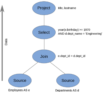
Data flows from the tables at the bottom upwards through the join, through the select, and finally through the project to produce the final results. The data passed between each node is logically a result set with columns and rows.
Of course, this is what happens logically , not how the plan is actually executed. Starting from this initial plan, the query planner performs transformations on the query plan tree to produce an equivalent plan that retrieves the same results faster. Both a federated query planner and a relational database planner deal with the same concepts and many of the same plan transformations. In this example, the criteria on the Departments and Employees tables will be pushed down the tree to filter the results as early as possible.
In both cases, the goal is to retrieve the query results in the fastest possible time. However, the relational database planner does this primarily by optimizing the access paths in pulling data from storage.
In contrast, a federated query planner is less concerned about storage access because it is typically pushing that burden to the data source. The most important consideration for a federated query planner is minimizing data transfer.
Access patterns are used on both physical tables and views to specify the need for criteria against a set of columns. Failure to supply the criteria will result in a planning error, rather than a run-away source query. Access patterns can be applied in a set such that only one of the access patterns is required to be satisfied.
Currently any form of criteria referencing an affected column may satisfy an access pattern.
In federated database systems pushdown refers to decomposing the user level query into source queries that perform as much work as possible on their respective source system. Pushdown analysis requires knowledge of source system capabilities, which is provided to Teiid though the Connector API. Any work not performed at the source is then processed in Federate's relational engine.
Based upon capabilities, Teiid will manipulate the query plan to ensure that each source performs as much joining, filtering, grouping, etc. as possible. In may cases, such as with join ordering, planning is a combination of standard relational techniques and, cost based and heuristics for pushdown optimization.
Criteria and join push down are typically the most important aspects of the query to push down when performance is a concern. See Query Plans on how to read a plan to ensure that source queries are as efficient as possible.
A special optimization called a dependent join is used to reduce the rows returned from one of the two relations involved in a multi-source join. In a dependent join, queries are issued to each source sequentially rather than in parallel, with the results obtained from the first source used to restrict the records returned from the second. Dependent joins can perform some joins much faster by drastically reducing the amount of data retrieved from the second source and the number of join comparisons that must be performed.
The conditions when a dependent join is used are determined by the query planner based on Section 14.2.1, “Access Patterns”, hints, and costing information.
Teiid supports hints to control dependent join behavior:
MAKEIND - indicates that the clause should be the independent side of a depedent join.
MAKEDEP - indicates that the clause should be the dependent side of a join.
MAKENOTDEP - prevents the clause from being the dependent side of a join.
Theses can be placed in either the OPTION clause or directly in the FROM clause . As long as all Section 14.2.1, “Access Patterns” can be met, the MAKEIND, MAKEDEP, and MAKENOTDEP hints override any use of costing information. MAKENOTDEP supersedes the other hints.
Tip
The MAKEDEP/MAKEIND hint should only be used if the proper query plan is not chosen by default. You should ensure that your costing information is representative of the actual source cardinality. An inappropriate MAKEDEP/MAKEIND hint can force an inefficient join structure and may result in many source queries.
The engine will for IN clauses to filter the values coming from the dependent side. If the number of values from the independent side exceeds the translators MaxInCriteriaSize, the values will be split into multiple IN predicates up to MaxDependentPredicates. When the number of independent values exceeds MaxInCriteriaSize*MaxDependentPredicates, then multiple dependent queries will be issued in parallel.
Copy criteria is an optimization that creates additional predicates based upon combining join and where clause criteria. For example, equi-join predicates (source1.table.column = source2.table.column) are used to create new predicates by substituting source1.table.column for source2.table.column and vice versa. In a cross source scenario, this allows for where criteria applied to a single side of the join to be applied to both source queries
Teiid ensures that each pushdown query only projects the symbols required for processing the user query. This is especially helpful when querying through large intermediate view layers.
Partial aggregate pushdown allows for grouping operations above multi-source joins and unions to be decomposed so that some of the grouping and aggregate functions may be pushed down to the sources.
The optional join hint indicates to the optimizer that a joined table should be omitted if none of its columns are used by the output of the user query or in a meaningful way to construct the results of the user query. This hint is typically only used in view layers containing multi-source joins.
The optional join hint is applied as a comment on a join clause. It can be applied in both ANSI and non-ANSI joins. With non-ANSI joins an entire joined table may be marked as optional.
Example 14.2. Example Optional Join Hint
select a.column1, b.column2 from a, /*+ optional */ b WHERE a.key = b.key
Suppose this example defines a view layer X. If X is queried in such a way as to not need b.column2, then the optional join hint will cause b to be omitted from the query plan. The result would be the same as if X were defined as:
select a.column1 from a
Example 14.3. Example ANSI Optional Join Hint
select a.column1, b.column2, c.column3 from /*+ optional */ (a inner join b ON a.key = b.key) INNER JOIN c ON a.key = c.key
In this example the ANSI join syntax allows for the join of a and b to be marked as optional. Suppose this example defines a view layer X. Only if both column a.column1 and b.column2 are not needed, e.g. "SELECT column3 FROM X" will the join be removed.
The optional join hint will not remove a bridging table that is still required.
Example 14.4. Example Briding Table
select a.column1, b.column2, c.column3 from /*+ optional */ a, b, c WHERE ON a.key = b.key AND a.key = c.key
Suppose this example defines a view layer X. If b.column2 or c.column3 are solely required by a query to X, then the join on a be removed. However if a.column1 or both b.column2 and c.column3 are needed, then the optional join hint will not take effect.
Tip
When a join clause is omitted via the optional join hint, the relevant criteria is not applied. Thus it is possible that the query results may not have the same cardinality or even the same row values as when the join is fully applied.
Left/right outer joins where the inner side values are not used and whose rows under go a distinct operation will automatically be treated as an optional join and do not require a hint.
Example 14.5. Example Unnecessary Optional Join Hint
select a.column1, b.column2 from a LEFT OUTER JOIN /*+optional*/ b ON a.key = b.key
Warning
A simple "SELECT COUNT(*) FROM VIEW" against a view where all join tables are marked as optional will not return a meaningful result.
Union partitioning is inferred from the transformation/inline view. If one (or more) of the UNION columns is defined by constants and/or has WHERE clause IN predicates containing only constants that make each branch mutually exclusive, then the UNION is considered partitioned. UNION ALL must be used and the UNION cannot have a LIMIT, WITH, or ORDER BY clause (although individual branches may use LIMIT, WITH, or ORDER BY). Partitioning values should not be null. For example the view definition "select 1 as x, y from foo union all select z, a from foo1 where z in (2, 3)" would be considered partitioned on column x, since the first branch can only be the value 1 and the second branch can only be the values 2 or 3. Note that more advanced or explicit partition could be considered in the future. The concept of a partitioned union is used for performing partition-wise joins, in Chapter 7, Updatable Views, and Section 14.2.6, “Partial Aggregate Pushdown”.
Teiid also incorporates many standard relational techniques to ensure efficient query plans.
Rewrite analysis for function simplification and evaluation.
Boolean optimizations for basic criteria simplification.
Removal of unnecessary view layers.
Removal of unnecessary sort operations.
Advanced search techniques through the left-linear space of join trees.
Parallelizing of source access during execution.
EXISTS subqueries are typically rewrite to "SELECT 1 FROM ..." to prevent unnecessary evaluation of SELECT expressions.
Quantified compare SOME subqueries are always turned into an equivalent IN prediate or comparison against an aggregate value. e.g. col > SOME (select col1 from table) would become col > (select min(col1) from table)
Uncorrelated EXISTs and scalar subquery that are not pushed to the source can be preevaluated prior to source command formation.
Correlated subqueries used in DETELEs or UPDATEs that are not pushed as part of the corresponding DELETE/UPDATE will cause Teiid to perform row-by-row compensating processing. This will only happen if the affected table has a primary key. If it does not, then an exception will be thrown.
WHERE or HAVING clause IN and EXISTs predicates can take the MJ (merge join), DJ (dependent join), or NO_UNNEST (no unnest) hints appearing just before the subquery. The MJ hint directs the optimizer to use a traditional, semijoin, or antisemijoin merge join if possible. The DJ is the same as the MJ hint, but additional directs the optimizer to use the subquery as the independent side of a dependent join if possible. The NO_UNNEST hint, which supercedes the other hints, will direct the optimizer to leave the subquery in place.
Example 14.6. Merge Join Hint Usage
SELECT col1 from tbl where col2 IN /*+ MJ */ (SELECT col1 FROM tbl2)
Example 14.7. Dependent Join Hint Usage
SELECT col1 from tbl where col2 IN /*+ DJ */ (SELECT col1 FROM tbl2)
Example 14.8. No Unnest Hint Usage
SELECT col1 from tbl where col2 IN /*+ NO_UNNEST */ (SELECT col1 FROM tbl2)
The system property org.teiid.subqueryUnnestDefault controls whether the optimizer will by default unnest subqueries. The default is false. If true, then most non-negated WHERE or HAVING clause non-negated EXISTS or IN subquery predicates can be converted to a traditional merge join or as antijoin or semijoin variants.
WHERE clause EXISTs and IN predicates that can be rewriten to a traditional join with the semantics of the semi-join can preserved if the system property org.teiid.subqueryUnnestDefault is set to true or the subquery has a MJ hint.
EXISTs and scalar subqueries that are not pushed down, and not converted to merge joins, are implicitly limited to 1 and 2 result rows respectively.
Conversion of subquery predicates to nested loop joins is not yet available.
A technique known as document projection is used to reduce the memory footprint of the context item document. Document projection loads only the parts of the document needed by the relevant XQuery and path expressions. Since document projection analysis uses all relevant path expressions, even 1 expression that could potentially use many nodes, e.g. //x rather than /a/b/x will cause a larger memory footprint. With the relevant content removed the entire document will still be loaded into memory for processing. Document projection will only be used when there is a context item (unnamed PASSING clause item) passed to XMLTABLE/XMLQUERY. A named variable will not have document projection performed. In some cases the expressions used may be too complex for the optimizer to use document projection. You should check the SHOWPLAN DEBUG full plan output to see if the appropriate optimization has been performed.
With additional restrictions, simple context path expressions allow the processor to evaluate document subtrees independently - without loading the full document in memory. A simple context path expression can be of the form "[/][ns:]root/[ns1:]elem/...", where a namespace prefix or element name can also be the * wild card. As with normal XQuery processing if namespace prefixes are used in the XQuery expression, they should be declared using the XMLNAMESPACES clause.
Example 14.9. Streaming Eligible XMLQUERY
XMLQUERY('/*:root/*:child' PASSING doc)Rather than loading the entire doc in-memory as a DOM tree, each child element will be independently added to the result.
Example 14.10. Streaming Ineligible XMLQUERY
XMLQUERY('//child' PASSING doc)The use of the descendent axis prevents the streaming optimization, but document projection can still be performed.
When using XMLTABLE, the COLUMN PATH expressions have additional restrictions. They are allowed to reference any part of the element subtree formed by the context expression and they may use any attribute value from their direct parentage. Any path expression where it is possible to reference a non-direct ancestor or sibling of the current context item prevent streaming from being used.
Example 14.11. Streaming Eligible XMLTABLE
XMLTABLE('/*:root/*:child' PASSING doc COLUMNS fullchild XML PATH '.', parent_attr string PATH '../@attr', child_val integer)The context XQuery and the column path expression allow the streaming optimization, rather than loading the entire doc in-memory as a DOM tree, each child element will be independently added to the result.
Example 14.12. Streaming Ineligible XMLTABLE
XMLTABLE('/*:root/*:child' PASSING doc COLUMNS sibling_attr string PATH '../other_child/@attr')The reference of an element outside of the child subtree in the sibling_attr path prevents the streaming optimization from being used, but document projection can still be performed.
Teiid provides the capability to obtain "partial results" in the event of data source unavailability or failure. This is especially useful when unioning information from multiple sources, or when doing a left outer join, where you are 'appending' columns to a master record but still want the record if the extra information is not available.
A source is considered to be 'unavailable' if the connection factory associated with the source issues an exception in response to a query. The exception will be propagated to the query processor, where it will become a warning on the statement. See the Client Guide for more on Partial Results Mode and SQLWarnings.
When integrating information using a federated query planner, it is useful to be able to view the query plans that are created, to better understand how information is being accessed and processed, and to troubleshoot problems.
A query plan is a set of instructions created by a query engine for executing a command submitted by a user or application. The purpose of the query plan is to execute the user's query in as efficient a way as possible.
You can get a query plan any time you execute a command. The SQL options available are as follows:
SHOWPLAN [ON|DEBUG]- Returns the plan or the plan and the full planner debug log.
With the above options, the query plan is available from the
Statement object by casting to the
org.teiid.jdbc.TeiidStatement
interface.
Example 14.13. Retrieving a Query Plan
statement.execute("set showplan on");
ResultSet rs = statement.executeQuery("select ...");
TeiidStatement tstatement = statement.unwrap(TeiidStatement.class);
PlanNode queryPlan = tstatement.getPlanDescription();
System.out.println(queryPlan);
The query plan is made available automatically in several of Teiid's tools.
Once a query plan has been obtained you will most commonly be looking for:
Source pushdown -- what parts of the query that got pushed to each source
Join ordering
Join algorithm used - merge or nested loop.
Presence of federated optimizations, such as dependent joins.
Join criteria type mismatches.
All of these issues presented above will be present subsections of the plan that are specific to relational queries. If you are executing a procedure or generating an XML document, the overall query plan will contain additional information related the surrounding procedural execution.
A query plan consists of a set of nodes organized in a tree structure. As with the above example, you will typically be interested in analyzing the textual form of the plan.
In a procedural context the ordering of child nodes implies the order of execution. In most other situation, child nodes may be executed in any order even in parallel. Only in specific optimizations, such as dependent join, will the children of a join execute serially.
Relational plans represent the actually processing plan that is composed of nodes that are the basic building blocks of logical relational operations. Physical relational plans differ from logical relational plans in that they will contain additional operations and execution specifics that were chosen by the optimizer.
The nodes for a relational query plan are:
Access - Access a source. A source query is sent to the connection factory associated with the source. [For a dependent join, this node is called Dependent Select.]
Project - Defines the columns returned from the node. This does not alter the number of records returned. [When there is a subquery in the Select clause, this node is called Dependent Project.]
Project Into - Like a normal project, but outputs rows into a target table.
Select - Select is a criteria evaluation filter node (WHERE / HAVING). [When there is a subquery in the criteria, this node is called Dependent Select.]
Join - Defines the join type, join criteria, and join strategy (merge or nested loop).
Union - There are no properties for this node, it just passes rows through from it's children
Sort - Defines the columns to sort on, the sort direction for each column, and whether to remove duplicates or not.
Dup Removal - Same properties as for Sort, but the removeDups property is set to true
Group - Groups sets of rows into groups and evaluates aggregate functions.
Null - A node that produces no rows. Usually replaces a Select node where the criteria is always false (and whatever tree is underneath). There are no properties for this node.
Plan Execution - Executes another sub plan.
Limit - Returns a specified number of rows, then stops processing. Also processes an offset if present.
Every node has a set of statistics that are output. These can be used to determine the amount of data flowing through the node.
|
Statistic |
Description |
Units |
|---|---|---|
|
Node Output Rows |
Number of records output from the node |
count |
|
Node Process Time |
Time processing in this node only |
millisec |
|
Node Cumulative Process Time |
Elapsed time from beginning of processing to end |
millisec |
|
Node Cumulative Next Batch Process Time |
Time processing in this node + child nodes |
millisec |
|
Node Next Batch Calls |
Number of times a node was called for processing |
count |
|
Node Blocks |
Number of times a blocked exception was thrown by this node or a child |
count |
In addition to node statistics, some nodes display cost estimates computed at the node.
|
Cost Estimates |
Description |
Units |
|---|---|---|
|
Estimated Node Cardinality |
Estimated number of records that will be output from the node; -1 if unknown |
count |
For each sub-command in the user command an appropriate kind of sub-planner is used (relational, XML, procedure, etc).
Each planner has three primary phases:
Generate canonical plan
Optimization
Plan to process converter - converts plan data structure into a processing form
The GenerateCanonical class generates the initial (or “canonical” plan). This plan is based on the typical logical order that a SQL query gets executed. A SQL select query has the following possible clauses (all but SELECT are optional): SELECT, FROM, WHERE, GROUP BY, HAVING, ORDER BY, LIMIT. These clauses are logically executed in the following order:
FROM (read and join all data from tables)
WHERE (filter rows)
GROUP BY (group rows into collapsed rows)
HAVING (filter grouped rows)
SELECT (evaluate expressions and return only requested columns)
INTO
ORDER BY (sort rows)
LIMIT (limit result set to a certain range of results)
These clauses translate into the following types of planning nodes:
FROM: Source node for each from clause item, Join node (if >1 table)
WHERE: Select node
GROUP BY: Group node
HAVING: Select node
SELECT: Project node and DupRemoval node (for SELECT DISTINCT)
INTO: Project node with a SOURCE Node
ORDER BY: Sort node
LIMIT: Limit node
UNION, EXCEPT, INTERSECT: SetOp Node
There is also a Null Node that can be created as the result of rewrite or planning optimizations. It represents a node that produces no rows
Relational optimization is based upon rule execution that evolves the initial plan into the execution plan. There are a set of pre-defined rules that are dynamically assembled into a rule stack for every query. The rule stack is assembled based on the contents of the user’s query and its transformations. For example, if there are no view layers, then RuleMergeVirtual, which merges view layers together, is not needed and will not be added to the stack. This allows the rule stack to reflect the complexity of the query.
Logically the plan node data structure represents a tree of nodes where the source data comes up from the leaf nodes (typically Access nodes in the final plan), flows up through the tree and produces the user’s results out the top. The nodes in the plan structure can have bidirectional links, dynamic properties, and allow any number of child nodes. Processing plan nodes in contrast typical have fixed properties, and only allow for binary operations - due to algorithmic limitations.
Below are some of the rules included in the planner:
RuleRemoveSorts - removes sort nodes that do not have an effect on the result. This most common when a view has an non-limited ORDER BY.
RulePlaceAccess - insert an Access node above every physical Source node. The source node represents a table typically. An access node represents the point at which everything below the access node gets pushed to the source. Later rules focus on either pushing stuff under the access or pulling the access node up the tree to move more work down to the data sources. This rule is also responsible for placing Section 14.2.1, “Access Patterns”.
RulePushSelectCriteria - pushes select criteria down through unions, joins, and views into the source below the access node. In most cases movement down the tree is good as this will filter rows earlier in the plan. We currently do not undo the decisions made by PushSelectCriteria. However in situations where criteria cannot be evaluated by the source, this can lead to sub optimal plans.
One of the most important optimization related to pushing criteria, is how the criteria will be pushed trough join. Consider the following plan tree that represents a subtree of the plan for the query "select ... from A inner join b on (A.x = B.x) where A.y = 3"
          SELECT (B.y = 3)
           |
          JOIN - Inner Join on (A.x = B.x
         /     \
      SRC (A)   SRC (B)
Note: SELECT nodes represent criteria, and SRC stands for SOURCE.
It is always valid for inner join and cross joins to push (single source) criteria that are above the join, below the join. This allows for criteria originating in the user query to eventually be present in source queries below the joins. This result can be represented visually as:
          JOIN - Inner Join on (A.x = B.x)
          /    \
         /   SELECT (B.y = 3)
        |        |
      SRC (A)   SRC (B)
The same optimization is valid for criteria specified against the outer side of an outer join. For example:
          SELECT (B.y = 3)
           |
          JOIN - Right Outer Join on (A.x = B.x)
         /     \
      SRC (A)   SRC (B)
Becomes
          JOIN - Right Outer Join on (A.x = B.x)
          /    \
         /   SELECT (B.y = 3)
        |        |
      SRC (A)   SRC (B)
However criteria specified against the inner side of an outer join needs special consideration. The above scenario with a left or full outer join is not the same. For example:
          SELECT (B.y = 3)
           |
          JOIN - Left Outer Join on (A.x = B.x)
         /     \
      SRC (A)   SRC (B)
Can become (available only after 5.0.2):
          JOIN - Inner Join on (A.x = B.x)
          /    \
         /   SELECT (B.y = 3)
        |        |
      SRC (A)   SRC (B)
Since the criterion is not dependent upon the null values that may be populated from the inner side of the join, the criterion is eligible to be pushed below the join – but only if the join type is also changed to an inner join.
On the other hand, criteria that are dependent upon the presence of null values CANNOT be moved. For example:
          SELECT (B.y is null)
           |
          JOIN - Left Outer Join on (A.x = B.x)
         /     \
      SRC (A)   SRC (B)
This plan tree must have the criteria remain above the join, since the outer join may be introducing null values itself. This will be true regardless of which version of Teiid is used.
RulePushNonJoinCriteria - this rule will push criteria out of an on clause if it is not necessary for the correctness of the join.
RuleRaiseNull - this rule will raise null nodes to their highest possible point. Raising a null node removes the need to consider any part of the old plan that was below the null node.
RuleMergeVirtual - merges view layers together. View layers are connected by nesting canonical plans under source leaf nodes of the parent plan. Each canonical plan is also sometimes referred to as a “query frame”. RuleMergeVirtual attempts to merge child frames into the parent frame. The merge involves renaming any symbols in the lower frame that overlap with symbols in the upper frame. It also involves merging the join information together.
RuleRemoveOptionalJoins - removes optional join nodes form the plan tree as soon as possible so that planning will be more optimal.
RulePlanJoins - this rule attempts to find an optimal ordering of the joins performed in the plan, while ensuring that Section 14.2.1, “Access Patterns” dependencies are met. This rule has three main steps. First it must determine an ordering of joins that satisfy the access patterns present. Second it will heuristically create joins that can be pushed to the source (if a set of joins are pushed to the source, we will not attempt to create an optimal ordering within that set. More than likely it will be sent to the source in the non-ANSI multi-join syntax and will be optimized by the database). Third it will use costing information to determine the best left-linear ordering of joins performed in the processing engine. This third step will do an exhaustive search for 6 or less join sources and is heuristically driven by join selectivity for 7 or more sources.
RuleCopyCriteria - this rule copies criteria over an equality criteria that is present in the criteria of a join. Since the equality defines an equivalence, this is a valid way to create a new criteria that may limit results on the other side of the join (especially in the case of a multi-source join).
RuleCleanCriteria - this rule cleans up criteria after all the other rules.
RuleMergeCriteria - looks for adjacent criteria nodes and merges them together. It looks for adjacent identical conjuncts and removes duplicates.
RuleRaiseAccess - this rule attempts to raise the Access nodes as far up the plan as possible. This is mostly done by looking at the source’s capabilities and determining whether the operations can be achieved in the source or not.
RuleChooseDependent - this rule looks at each join node and determines whether the join should be made dependent and in which direction. Cardinality, the number of distinct values, and primary key information are used in several formulas to determine whether a dependent join is likely to be worthwhile. The dependent join differs in performance ideally because a fewer number of values will be returned from the dependent side. Also, we must consider the number of values passed from independent to dependent side. If that set is larger than the max number of values in an IN criteria on the dependent side, then we must break the query into a set of queries and combine their results. Executing each query in the connector has some overhead and that is taken into account. Without costing information a lot of common cases where the only criteria specified is on a non-unique (but strongly limiting) field are missed. A join is eligible to be dependent if:
there is at least one equi-join criterion, i.e. tablea.col = tableb.col
the join is not a full outer join and the dependent side of the join is on the inner side of the join
The join will be made dependent if one of the following conditions, listed in precedence order, holds:
There is an unsatisfied access pattern that can be satisfied with the dependent join criteria
The potential dependent side of the join is marked with an option makedep
(4.3.2) if costing was enabled, the estimated cost for the dependent join (5.0+ possibly in each direction in the case of inner joins) is computed and compared to not performing the dependent join. If the costs were all determined (which requires all relevant table cardinality, column ndv, and possibly nnv values to be populated) the lowest is chosen.
If key metadata information indicates that the potential dependent side is not “small” and the other side is “not small” or (5.0.1) the potential dependent side is the inner side of a left outer join.
Dependent join is the key optimization we use to efficiently process multi-source joins.
Instead of reading all of source A and all of source B and joining them on A.x = B.x, we read all of A then build a set of A.x that are passed as a criteria when querying B. In cases where A is small and B is large, this can drastically reduce the data retrieved from B, thus greatly speeding the overall query.
RuleChooseJoinStrategy - Determines the base join strategy. Currently this is a decision as to whether to use a merge join rather than the default strategy, which is a nested loop join. Ideally the choice of a hash join would also be evaluated here. Also costing should be used to determine the strategy cost.
RuleDecomposeJoin - this rule perfomrs a partition-wise join optimization on joins of Section 14.2.8, “Partitioned Union”. The decision to decompose is based upon detecting that each side of the join is a partitioned union (note that non-ansi joins of more than 2 tables may cause the optimization to not detect the appropriate join). The rule currently only looks for situations where at most 1 partition matches from each side.
RuleCollapseSource - this rule removes all nodes below an Access node and collapses them into an equivalent query that is placed in the Access node.
RuleAssignOutputElements - this rule walks top down through every node and calculates the output columns for each node. Columns that are not needed are dropped at every node. This is done by keeping track of both the columns needed to feed the parent node and also keeping track of columns that are “created” at a certain node.
RuleValidateWhereAll - this rule validates a rarely used model option.
RuleAccessPatternValidation - validates that all access patterns have been satisfied.
RulePushLimit - pushes limit and offset information as far as possible in the plan.
The procedure planner is fairly simple. It converts the statements in the procedure into instructions in a program that will be run during processing. This is mostly a 1-to-1 mapping and very little optimization is performed.
The XML Planner creates an XML plan that is relatively close to the end result of the Procedure Planner – a program with instructions. Many of the instructions are even similar (while loop, execute SQL, etc). Additional instructions deal with producing the output result document (adding elements and attributes).
The XML planner does several types of planning (not necessarily in this order):
- Document selection - determine which tags of the virtual document should be excluded from the output document. This is done based on a combination of the model (which marks parts of the document excluded) and the query (which may specify a subset of columns to include in the SELECT clause).
- Criteria evaluation - breaks apart the user’s criteria, determine which result set the criteria should be applied to, and add that criteria to that result set query.
- Result set ordering - the query’s ORDER BY clause is broken up and the ORDER BY is applied to each result set as necessary
- Result set planning - ultimately, each result set is planned using the relational planner and taking into account all the impacts from the user’s query
- Program generation - a set of instructions to produce the desired output document is produced, taking into account the final result set queries and the excluded parts of the document. Generally, this involves walking through the virtual document in document order, executing queries as necessary and emitting elements and attributes.
XML programs can also be recursive, which involves using the same document fragment for both the initial fragment and a set of repeated fragments (each a new query) until some termination criteria or limit is met.